
In many cases the information in the section "Regression Diagnostics" is copy/pasted from the packages documentation in CRAN or other web sites.
- Correlation(X,Y)
- Linear Regression
- Model Assumptions
- Computing the linear regression
- Useful Functions
- Outstanding Observations
- Regression Diagnostics
Correlation(X,Y)
The Correlation Coefficient (just the correlation from now on) tell us how strength is the linear relationship between X and Y. The correlation is commutative and indifferent to the scale and displacement of X or Y. We can compute the correlation using the R function cor().
# Correlation Properties
cor(X, Y) = cor(Y, X)
cor(a*X, b*Y) = cor(X, Y)
cor(X + h, Y + k) = cor(X, Y)
cor(a*X + h, b*Y + k) = cor(X, Y)
Where X and Y are vectors with the same length and a, b, h and k are scalar constants.
The Correlation is a dimensionless value in the range [-1, 1]. Positive values are an indication that both variables are positively related: when one changes in one direction (increases or decreases) the other variable changes in the same way. Negative values indicate they are negatively related, when one changes in one way the other changes in the other way. The closer the correlation is to 1 or -1 the is stronger the linear relationship between X and Y.
The correlation close to zero or even zero, does not necessarily means that X and Y are not related. It only implies they are not linearly correlated. Furthermore, as many summary statistics it can be strongly influenced by one or a small set the outliers points in the data.
| X | Y |
|---|---|
| 0.5579 | 7.5412 |
| 1.4529 | 13.4511 |
| 2.4536 | 23.5669 |
| 3.2209 | 37.8855 |
| 4.365 | 50.9916 |
| 5.3777 | 71.4575 |
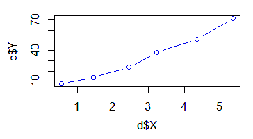
plot(d$X, d$Y, type=b, col=blue)
With the example data in the table above (dataframe 'd'), we will compute the correlation between Y and some power functions of X.
> cor(d$X, d$Y)
[1] 0.9879264

> cor(d$X^1.5, d$Y)
[1] 0.9976092

> cor(d$X^2, d$Y)
[1] 0.9928579
Linear Regression
In a linear regression there is a model expressing a linear relationship between the response or dependent variable and one or more predictor variables. The number of predictor variables is denoted with the term "p", the number of coefficients is denoted with the term "c". When there is an interception or constant in the model c = p + 1 but when there is not such interception c = p. The number of data points or observations used in the regression is "n".
    Y = β₀ + β₁⋅X₁ + ... + βp⋅Xp + ε
    ε ~ Ν(0, σ²)
Where ε is the error, a random variable (in consequence Y is also a random variable), with constant variance and mean zero (see the following assumptions). This error is estimated by the regression residuals, but they are not the same thing.
Model Assumptions
1) Linearity
The relationships between the predictors and the response variable should be linear.
2) The predictor variables are not non-random
The values of the predictor variables are fixed or selected in advance. A consequence of this assumption is the predictor values are are measured without error: if there would be a random error in the measurement of the predictor, it would be random variables!
The consequence of failing this assumption depends —most importantly— on the magnitude of the measurement Variance and the correlation among the predictor errors. If the measurement errors are small with respect to the random errors, their effect in the regression is slight.
3) The predictor variables are linearly independent of each other
This is also referred as lack of multicolinearity in the predictors. This is easy to understand supposing we pretend to have a model with two predictors where in fact the predictors are linearly related to each other. In such case, we have only one predictor! This condition is easy to validate testing the correlation between the predictors.
4) The error has a Normal distribution
The errors should be normally distributed. This is usually called the normality assumption. Technically this is necessary only for valid hypothesis testing, the estimation of the coefficients only requires that the errors be identically and independently distributed.
5) The errors has mean zero
6) The errors has the same Variance
The Variance, and in consequence the Standard Deviation, of the errors is constant: For example, it does not depends on a predictor value. This property is called homoscedasticity and when this assumption does not hold it is called heteroscedasticity.
When there is heteroscedasticity, the simple linear regression (OLS) give less precise parameter estimates and misleading standard errors.
7) The errors are independent of each other
The errors are not correlated to each other. This is also called the independent-error assumption when this assumption does not hold there is an auto correlation problem.
Computing the linear regression
We can compute the OLS (Ordinary Least Squares) linear regression using the lm() function. For example, we will use it with the data shown above, then we will call the summary() function to get a rather standard presentation of the regression found by R:
# Simple OLS
lr = lm(y ~ x1 + x2, data=df)

# Get the regression with intercept equal to zero.
lr = lm(y ~ x1 + x2 + 0)

# WLS (weighted) regression
lr = <- rlm(y ~ x1 + x2, data=df, weight=w)

# Robust (and weighted) regression
library(robustbase)
lr = lmrob(y ~ x1 + x2, data=df, weight=w)
Get the regression summary information:
summary(lr)
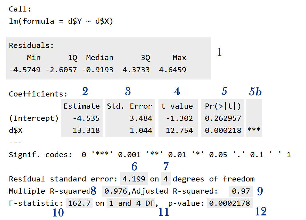
Output of regression summary()
We have the following information:
1) A summary of the residuals (ε).
Each residual is the difference between the real measured Y response value and the estimated (fitted) Y according to the regression. This corresponds to the ε term in the model.
2) The estimated value of each coefficient (βi).
If the coefficient is zero it means the predictor variable is not related to the response variable, it is not useful to explain or predict its behavior. Therefore, we have to ask ourselves how statistically significant is each coefficient? This is answered with the data in the point (5).
We can get the just the regression coefficients with the function coef().
> coef(lr)
(Intercept)         d$X
  -4.534706   13.317767
3) The estimated Standard Error or Standard Deviation of each coefficient.
The smaller the error, the greatest the accuracy of the estimated coefficient.
We can get the coefficients confident intervals with the function confint(). By default confint() computes the confidence intervals with a confidence level of 95% but we can change this with the level parameter.
> confint(lr)
                2.5 %    97.5 %
(Intercept) -14.20774  5.138325
d$X          10.41852 16.217008

> confint(lr, level=0.9)
                  5 %      95 %
(Intercept) -11.96198  2.892568
d$X          11.09163 15.543901
4) The t value of each coefficient.
Under the normality assumption about the residuals. The quotient of each coefficient divided by its standard error follows a t Student's distribution. This allow us to test the null hypothesis H₀: "The coefficient is zero", against the alternative, H₁: "The coefficient is not zero". See the following point (5).
5) Each coefficient p-value.
This is the value we can directly use to reject or not the hypothesis about the corresponding coefficient being zero (or not) as expressed in (4). This is the probability to get the given coefficient by chance alone. If this probability is below to a given significance level, the null hypothesis H₀: "The coefficient is zero" can be rejected.
In the summary shown above, for a 5% significance level, the null hypothesis can not be rejected for the interception (26.2957 > 5%). This means there is a 26.2957% chance to get, for this coefficient, a non zero estimation just by chance; with that chance this interception could be zero and the model consideration about having this non-zero interception adds nothing to tit.
However, for the line slope —the coefficient for d$X— the null hypothesis can be rejected (0.02178% < 5%). This means "d$X" is a statistically significant predictor of "d$Y". The probability to get this coefficient "just by chance" is 0.0218%: around 2 in 10,000!
5b) This is a key indicating how great is the certainty that the corresponding coefficient is not zero. The legend below the coefficients summary explain their meaning. You can suppress this key using the following command:
> options(show.signif.stars=FALSE)
6) The residuals standard error.
The Standard Deviation (σ) of the residual errors.
7) The degrees of freedom of the residuals standard errors.
This is the number of observations (data points) minus the number of coefficients in the regression model.
8) The (unadjusted) Coefficient of Determination R².
This value measures the model quality and is in the range [0, 1], where bigger means a better. Technically, this is the fraction of the Variance of Y explained by the regression model.
Warning: R² doesn’t make any sense if you do not have an intercept in your model. This is because the denominator in the definition of ² has a null model with an intercept in mind when the sum of squares is calculated. Beware of high R2s reported from models without an intercept.
9) The adjusted Coefficient of Determination R².
This coefficient is smaller than and derived from the unadjusted R² (8). This coefficient takes into account the number of coefficients in the regression. If two regressions have the same value for the unadjusted R² (8), the regression with the lesser number of coefficients, will have the better adjusted R². It is more realistic and effective use this Coefficient of Determination instead of the unadjusted one.
R² = (cor(d$X, d$Y))²
R² = (0.9879264)²
R² = 0.97599
10) The F statistic for the whole model.
See (11) and (12).
11) The degrees of freedom corresponding to the F statistic given in (10).
12) The probability value (p-value) corresponding to (10) and (11).
This statistic tell us if the model is significant or not.
In a similar way as the coefficients p-values, this one can be used to validate the whole model. If this value is smaller than a given significance level, the model is significant —at that level— otherwise, the model is not significant and the predictor variables are not related to the response variable as described by the model.
If all the coefficients p-value —explained in (5)— are poor, this one —for the whole model— will be also poor. If any of the coefficients is nonzero the model is significant. It is more useful check this value and then check R².
Useful Functions
There are some useful functions directly related to linear regressions:
coef()
Returns the model coefficients.confint()
Returns the confidence intervals for one or more parameters in a fitted model.fitted()
Returns the fitted response values predicted by the model.resid(), residuals()
Returns the model residuals.deviance()
Returns the deviance or residual sum of squares.
Outstanding Observations
We want to be sure the regression coefficients are not unduly determined by a few observations describing a behavior or pattern very different to the other observations.
An observation is called influential when its removal (singly or in combination with few others) causes significant changes in the model, as the predictor coefficients, their standard errors, the Coefficient of Determination, etc.
We need the following definitions to deal with this.
Outliers
With respect to regression models, we must distinguish different kinds of outliers.
- There is outliers in their own domain (or space), called univariate outliers:
a) Outliers in the response domain.
b) Outliers in the predictor space.
For example, an observation with an unusual value for the response variable (Y) or an observation with an unusual value for one —or more— of the predictor variables (Xi).
- There is outliers in the regression model: a regression outlier is an observation with a large residual. This means with an unusual value for the response variable considering the corresponding predictor variable(s).
The Engineering Statistics Handbook distinguish mild outliers and extreme outliers and gives the method to find the borders (fences) to categorize the data as not outliers, mild outliers and extreme outliers:
lower outer fence = Q1 - 3*IQ
lower inner fence = Q1 - 1.5*IQ
upper inner fence = Q3 + 1.5*IQ
upper outer fence = Q3 + 3*IQ
Where a point beyond an inner fence on either side is considered a mild outlier. A point beyond an outer fence is considered an extreme outlier. IQ is the interquartile range and is the difference between (Q3 - Q1).
For example, using the output of the regression summary shown above, we have the following for the Residuals:
Q1 = -2.6057
Q3 = 4.3733
IQ = 4.3733 - -2.6057 = 6.979

lower outer fence = Q1 - 3*IQ   = -2.6057 -   3*6.979 = -23.54
lower inner fence = Q1 - 1.5*IQ = -2.6057 - 1.5*6.979 = -13.0742
upper inner fence = Q3 + 1.5*IQ =  4.3733 + 1.5*6.979 = 14.8418
upper outer fence = Q3 + 3*IQ   =  4.3733 +   3*6.979 = 25.3103
In summary, there are the following kind of outlier observations:
- Regression model outliers.
- Outliers in the predictor space.
- Outliers in the response domain.
When looking for influential points we are more interested in the first two cases.
It is important to consider that an outlier observation is not necessarily an influential point.
Leverage, leverage-value, high-leverage point
"Leverage" is an attribute of each observation, strongly related to its position in the predictor space, indicating its potential of being an influential point. In any regression diagnostic the points with high leverage should be flagged and analyzed to find how influential they are.
An observation must considered a high-leverage point when:
- The observation is an outlier in the predictor space.
- The observation statistic leverage-value is twice greater its average value.
Observations that are outliers in the predictor space are known as high-leverage points.
Every observation —used to calculate the regression— has an associated statistic called leverage-value. The leverage-value of an observation measures how much the the whole regression model would be moved if the observation point is moved one unit in the Y (response) direction.
The leverage-values lie in the range [0, 1]. Points with zero leverage-value has no effect on the regression model. If a point had a leverage-value equal to 1, the line would follow (chase) the point perfectly.
The average of leverage-values is (p + 1)/n. The observations with leverage-value greater than twice this average must be treated as high-leverage points.
Regression Diagnostics
Get the Regression Residuals
For a WLS regression, the residuals function does not return the residual considering the model weights. To get that is required to use the parameter type="pearson".
# This works fine for WLS and for OLS (weight=1)
resid <- residuals(lr,type="pearson")
studRes <- rstudent(lr)
standRes <- rstandard(lr)
Influential Observations
Cook Distance
cookDistTop <- 4/(length(gb$X)-length(fit$coefficients))
cookDist <- cooks.distance(fit)
#Look for values above cookDistTop
plot(fit, which=4, cook.levels=cookDistTop)

plot(gb$Mean, cookDist)
abline(h=cookDistTop)
identify(gb$Mean, cookDist, gb$ID)

#Look for outliers
halfnorm(cookDist, nlab=3, ylab="Cook's Distances")
Regression Diagnostics
This function provides the basic quantities which are used in forming a wide variety of diagnostics for checking the quality of regression fits.
library(stats)
influence(lr)
Influence Index Plot
Provides index plots of Cook's distances, Studentized residuals, Bonferroni p-values, and leverages (hat-vales).
library(car)
influenceIndexPlot(lr, id.method="identify")
Influence Plot
This function creates a “bubble” plot of Studentized residuals by hat values, with the areas of the circles representing the observations proportional to Cook's distances. Vertical reference lines are drawn at twice and three times the average hat value, horizontal reference lines at -2, 0, and 2 on the Studentized-residual scale.
library(car)
influencePlot(lr,   id.method="identify", main="Influence Plot", sub="Circle size is proportional to Cook's Distance" )
Hadi Index plot
Provides an index plot with Hadi's influence indices (Hi).
library(bstats)
influential.plot(fit, type="hadi", ID=TRUE)
Bonferroni Outlier Test
Reports the Bonferroni p-values for Studentized residuals in linear and generalized linear models, based on a t-test for linear models and normal-distribution test for generalized linear models.
> library(car)
> outlierTest(lr)

    rstudent unadjusted p-value Bonferonni p
10 -9.921681         1.3592e-21   8.2369e-19
6  -7.726827         4.6252e-14   2.8029e-11
12 -7.151427         2.4965e-12   1.5129e-09
Regression Leverage Plots
These functions display a generalization, due to Sall (1990) and Cook and Weisberg (1991), of added-variable plots to multiple-df terms in a linear model. When a term has just 1 df, the leverage plot is a rescaled version of the usual added-variable (partial-regression) plot.
# leverage plots
leveragePlots(fit)
Error Normality tests
Shapiro-Wilk test
shapiro.test(residuals(lr))
Q-Q plot for Studentized residuals
The Studentized residuals should have a Student's t-distribution with n-p-2 degrees of freedom. The qqPlot function draws a theoretical quantile-comparison plots for variables and for Studentized residuals from a linear model. A comparison line is drawn on the plot either through the quartiles of the two distributions, or by robust regression,with 95% confidence borders.
par(mar=c(4.9,4.8,2,2.1), cex=0.9, cex.axis=0.8)
qqPlot(fit, main="QQ Plot", id.n=4)
Q-Q plot for Normality of residuals
qqnorm(residuals(lr), ylab="Residuals")
qqline(residuals(lr))
Q-Q plot for Normality of standardized residuals
stdRes = rstandard(lr)
qqnorm(stdRes, ylab="Standardized Residuals")
abline(0, 1)
Heteroscedasticity Tests
Check the residuals spread level against fitted values.
Tries to fit the residuals spread level with the fitted values.
If the p-value of the regression is above a given significance level, the null hypothesis "The residuals magnitude are not significantly linearly correlated with the fitted values" can not be rejected. Check the spread-Level Plots below.
summary(lm(abs(residuals(lr)) ~ fitted(lr)))
bpTest Breusch-Pagan test for heteroscedasticity.
The test checks the hypothesis "The model variance is homoscedastic".
This test tries to relate, using a linear regression model, the square of the model residuals with the predictor variables (by default) or with the potential explanatory variables given in the parameter varformula. If the H₀ hypothesis: "The (square of) residuals can be predicted by the given explanatory variables —it is not constant—" holds, the statistic returned by the test follows a chi-squared distribution: If the p.value returned by the test is below a given confidence level, the null hypothesis can be rejected.
library(bstats)

# Test if the squared residuals are correlated with "X2"
bptest(model=Y ~ X + X2, varformula=~ X2 data=gb)

# Here "lr" is a fitted "lm" object.
bptest(model=lr)
ncvTest Breusch-Pagan test for heteroscedasticity.
This test is similar to bptest, but this function tries —by default— to relate the square of residuals with the fitted values, not with the predictors.
library(car)
ncvTest(lr)
Spread-Level Plots
Creates plots for examining the possible dependence of spread on level —or an extension of these plots— to the Studentized residuals from linear models.
For linear models, plots log(abs(studentized residuals) vs. log(fitted values).
For non linear models, computes the statistics for, and plots, a Tukey spread-level plot of log(hinge-spread) vs. log(median) for the groups; fits a line to the plot; and calculates a spread-stabilizing transformation from the slope of the line.
library(car)
spreadLevelPlot(lr)
Multi-collinearity
# Evaluate Collinearity
vif(fit) # variance inflation factors
sqrt(vif(fit)) > 2 # problem?
Nonlinearity
# Evaluate Nonlinearity
# component + residual plot
crPlots(fit)
# Ceres plots
ceresPlots(fit)
Non-independence of Errors
# Test for Autocorrelated Errors
durbinWatsonTest(fit)
Global test of model assumptions
library(gvlma)
gvmodel <- gvlma(fit)
summary(gvmodel)
Model Adequacy
test model adequacy.
Residual Plots and Curvature Tests for Linear Model Fits
The function residualPlots graphs the residuals against the predictors and the fitted value.
The function also computes a curvature test, for each of the plots, by adding a quadratic term and testing if the quadratic coefficient is zero. This is the Tukey's test for non-additivity. Stated in simple terms, the null hypothesis is "The data fits a linear model". If the fit is not bad, the p-value is big enough to do not reject the hypothesis.
library(car)
residualPlots(fit)
Marginal Model Plots
library(car)
marginalModelPlots(fit)
If the model fits the data well, then the two smooths should match on each of the marginal model plots; if any pair of smooths fails to match, then we have evidence that the model does not fit the data well.
Added-variable plots
The avPlots function constructs added-variable (also called partial-regression) plots for linear and generalized linear models.
avPlots(lr, id.n=3, col="darkgreen", bg="green", pch=21)