There is interesting information in the web depicting the behavior and noise characterization of a digital CMOS DSLR. For example this article about DSLR sensor noise behavior is very interesting and well known. In posts like these it is said —for example— in the image Variance (the square of the noise) the Shot Noise is a linear component (with respect to the signal) and the PRNU Noise is a quadratic one. However, there is not an explanation about how this behavior arises, even when the presented data clearly supports those affirmations.
With the desire of getting a mathematical model explaining why the aforementioned noise component has that given mathematical profile we have just used some properties of the statistical Variance and Expected Value on a simple sensor model and we have found some simple equations explaining the different noise components and the whole Photon Transfer Curve (the curve of the noise as response of the signal).
In this article we will develop that sensor model from the scratch. But we will give just simple definitions for the intervening elements. If you want more detail about them, please look in the web for those definitions. Here we will focus on the interplay between those elements from rather a theoretical point of view but also by using real data.
We will use the formulas and notation given in "Commonly Used Math Formulas: Statistics formulas".
The statistics formulas, referring to distribution parameters as the Expected Value or the Variance of a random variable, when used with estimators (computed from sample data as the average instead of the Expected Value) instead of the actual distribution parameters, help us both, to derive another estimator and to understand their relationship.
Formally, the relationship between those estimators and the relationship between the actual distribution parameters are usually represented with different notation and different equations. For example, the second equation below uses the "hat notation" for the estimators:

However, for the sake of simplicity, we will not make that differentiation, but understanding —as we already said— those formulas, when used with estimators, help us to get other estimators and to understand their expected relationship.
The Image Noise
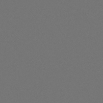
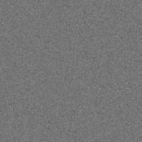
The image noise is random spikes of luminance change —in each of the RGB image channels— in places where it is expected to be uniform or maybe changing gradually. It is more noticeable in the dark areas and when the image is enlarged or closely inspected at pixel level. The noise can be described as composed by "luminance noise" and "color noise", where "luminance noise" is noise keeping basically the same overall hue and in "color noise" (also called "chroma noise") there is also changes in the hue. However, as the noise is random changes in the RGB channels, its presence in a raw image always involves both types of noise. Please see the following samples.


The image at the left has color and luminance noise, the one at the right has almost only luminance noise. Enlarged at 200%.
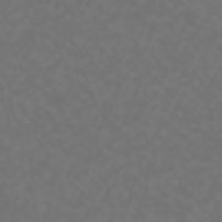
Besides creative or aesthetic intentions, the color noise is almost always undesirable. However, the luminance noise is not necessarily an unwanted image feature, sometimes it is required to avoid a posterized or plasticized look.


The image at the left has some luminance noise leaving some texture detail avoiding a plasticized look as the image at the right without any noise. However, this is hard to notice in retina displays.
As the noise is luminance change, it is best measured with the Standard Deviation statistic, which measures the amount of variation of values from their own average. From now to on, when referring to the noise amount, we will be talking about the Standard Deviation (it is usually represented with the Greek letter sigma "σ") of the luminosity along the image surface. In turn, the Standard Deviation is the square root of the Variance, which correspondingly is represented as the sigma squared "σ²". In other words, the noise is also the square root of the Variance.
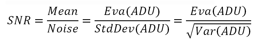
The human vision can resolve changes of luminosity when that change is above about 1%. Setting aside the value, this way to detect luminosity changes on the base of a contrast ratio, means that the same noise is more noticeable when the average luminosity is lower and is less noticeable —or not noticeable at all— when the average luminosity is higher. In turn this implies that the best way to measure the visual impact of the noise is considering the proportion between the Noise and the average luminosity of the image area containing the noise. The "classic" way to express this proportion is through the Signal to Noise ratio (usually abbreviated as S/N or SNR), this is the (arithmetic) mean or average luminosity divided by the amount of noise (Standard Deviation).
As the average luminosity and the Standard Deviation are both given in ADUs (Analog-to-Digital Unit: a dimensionless unit of measure, the raw image pixel values are said to be in ADUs), the SNR ratio is dimensionless.
It is implicit that the Mean and Standard Deviation are calculated among the pixels of the same image, over an area where all the pixels should have the same luminosity.
SNR = Mean_pixel_Luminosity / StdDev_pixel_Luminosity = Mean/Noise
As the noise are random changes and we measure it with the Standard Deviation , it is easy to see that the use of statistics will be useful to analyze it. In the practice we will approximate the luminosity Expected Value (denoted with the Eva() operator) with the image sample average luminosity and the Standard Deviation will be obtained from the image sample variance (denoted with the Var() operator).
We will compute those statistic values from raw image data, where the pixel values are in ADU units.
As the Signal to Noise ratio can have a very broad range of values, it is normally expressed by its logarithm. This is can be a base 2 logarithm, in which case it is said the SNR is expressed in stops.
SNR_Stops = Log₂(SNR) = Log₂(Mean/Noise)
The SNR ratio is often expressed in decibels (dB), in which case it is calculated as 20 times the base 10 logarithm of the SNR.
SNR_dB = 20⋅Log₁₀(SNR) = 20⋅Log₁₀(Mean/Noise)
In the following table we have the SNR categories that, according to DxO Mark, can be considered as a reference for good, poor and bad noise levels. They are expressed in the three forms: the ratio itself, in stops and in dB. Of course the borders between neighbor categories are blurry and seems to overlap because where one ends the other begins.
| Noise Category | Ratio | Stops | dB |
|---|---|---|---|
| Good when above to | 80 | 6.3 | 38 |
| Acceptable when above to | 40 | 5.32 | 32 |
| Non acceptable from and above to | 10 | 3.32 | 20 |
| Very bad when below of | 10 | 3.32 | 20 |
A change of 6 dB approximately corresponds to a factor of 2 over the SNR. For example, notice in the table above, how when the SNR in dB changes from 38 to 32 (6 dB) the SNR changes from 80 to 40, effectively corresponding to a factor of two. The same happens from 32dB to 20dB, there is a difference of 2⋅6dB = 12dB, corresponding to twice the factor 2 (2⋅2 = 4), and correspondingly the SNR drops from 40 to 10 (40/10 = 4).
The following gadget shows samples of show the noise levels in the table above. Some juggling is required to avoid the Gamma Correction distorting the desired SNR: they were prepared in linear sRGB and then the image was converted to sRGB without changing the image appearance.

During the image editing we must be careful not to drop the SNR, for example adding contrast in noisy shadowed areas. If in a linear space we just raise the whole image luminance multiplying it by a given factor, the SNR won't change: If M and N are the current mean and noise levels, the current SNR is M/N. Raising the all the luminosity levels through a line with slope f will change the luminosity to "f⋅M". However the SNR will not change, because the noise will also change to "f⋅N".
In raw image processing software, this kind of adjustment is made with the "Exposure Correction" control.
SNR = (f⋅M)/(f⋅N) = M/N
We have seen how an implicit Tone Curve and/or Gamma Correction is applied (sometimes automatically and unavoidably) over the raw image linear luminosity in image processing software and this can interact with our image editing and unexpectedly lower the SNR.
The SNR is not the single factor to consider with respect to noise. The SNR is almost as important as its spatial frequency: two images can have the same SNR, one with small size noise, evenly sparkled over the image (higher spatial frequency) and the other with noise composed by chunks of different luminosity (lower spatial frequency). Clearly the second kind of noise is worse than the first. Please check the samples below.
A healthy human eye, depending on the environment conditions (determining pupils size), can resolve from 50 or 60 cycles per degree (cy/deg) up to around 100 cy/deg, as it is shown in the following graph showing the average human eye MTF ("borrowed" from the Journal of Vision). You can read about OTF and MTF (Optical & Modulation Transfer Function) in this Wikipedia page. Let's recall the human starts to resolve contrast from about 1%, that's why the "gain" begins at 0.01.

Mean radial MTFs for pupil diameters from 2 to 6 mm.
For a given viewing distance we can get the cycle size using the following formula. A cycle is standardized at two image pixels (on screen) or dots (when printed).
Cycle_Lenght = 2⋅Distance⋅Tan(Degrees_per_Cycle/2)
Let's suppose we have an image with characteristic noise of 50 SNR and we have found this noise has a size of 1.7 pixels, this means cycles of 3.4 pixel/cycle. If we print that image at 600 dpi, each cycle will have a length of (25.4mm/inch)/(600pixel/inch)⋅3.4pixel/cycle = 0.144 mm/cycle. At a viewing distance of 45 cm this cycles are at a spatial frequency of 54.6 cycles/degree (calculated using the reverse of the formula above). If we look the average human eye MTF, with a pupil aperture of 4mm (for example) we will find for 54.6 cycles/degree a gain of 0.04 approximately. This means that a noise with a contrast ratio of 1:50 (50 SNR) will be attenuated to 0.04:50 (the gain is 0.04), "corresponding" to a noise of 62 dB, which wont be seen by the observer.
We can now understand how the image presentation resolution (pixels/mm), viewing distance, noise size, noise intensity (SNR) and viewing environment (pupil size) are important factors to determine the impact of the noise in the viewed image. To complicate even more the subject, the human eye response to the spatial frequency is different for monochromatic and white light.
The ISO standard 15739:2013 "Photography - Electronic still-picture imaging - Noise measurements" specifies how to make camera noise measurements taken into account all the aforementioned factors.
This article is focused on the DSLR camera noise characterizations, its components, and their mathematical relationship. It is like if we were always considering the worse case scenario where the existing noise is clearly visible, as with a MTF gain of 1.
A Simple DSLR Camera Sensor Math Model
As we have seen in previous posts, each camera sensor photosite is sensitive —mainly— to only one of the RGB (red, green and blue) color components that will compose the final image. The following picture describes in simple but a meaningful way how the DSLR camera sensor converts the light hitting it to RGB pixel values in ADUs.

Photosites processing the light hitting it.
The light hitting the sensor during the exposition time, can be described as comprised by photons. When each photon reaches a particular layer on the sensor silicon, the photon produces an electron. The unit for a quantity of electrons is "e-".
Once the exposition time has end, the ADC (Analog to Digital Converter a.k.a. A/D Converter) in the photosite circuitry "counts" how many electrons are in each photosite and converts that count to ADUs. In this electron quantization, we will say, the ADC uses a conversion factor "M" (from Multiplier), with the unit "ADU/e-", to multiply the tally of electrons and get the corresponding ADU value. Before the exposition time begins, all of the photosites are reseted in order to start the exposition with their electronAPS count set to zero.
The "M" rate depends only the ISO speed setting of the camera. For higher ISO values, "M" will be higher, requiring fewer electrons to make an ADU, resulting in a more light sensitive sensor as expected.
The flux of the photons hitting each photosite is proportional to the intensity of the light originating the photons. This way —as expected— the darker areas of the photographed scene will correspond to a low count of electrons and in consequence low ADU values, whilst the brighter areas will correspond to higher ADU values. We will represent the count of electrons in each photosite —at the end of the exposition time— with the symbol "EL" (for ELectrons) and using the unit e-.
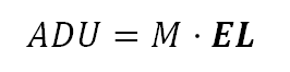
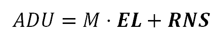
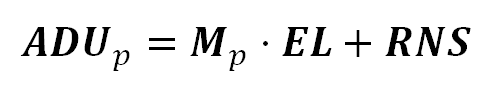
So far, our model for the sensor is:
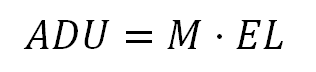
Formula 1. Model Prototype
Photon Shot Noise
Up to this point of our model, at first glance it seems we still don't have a source of noise, but we already have it, and it is the count of electrons represented by "EL".
Even with a perfectly uniform illumination, the count of electrons in each photosite —after the exposition— is not the same. That count instead of a constant is a random variable; those different values on the image surface are the kind of noise called the Photon Shot Noise.
To understand this, let's imagine a lot of identical mugs set under a uniform rain and that at the end of the rain no mug was overflown.

Rain as a Poisson Process.
If after the rain, we check the mugs, we will find that the amount of rain collected in each mug is not very different from the others. But if we measure it very precisely, we will find different amounts of rain in each mug. Something similar occurs with the photons hitting the photosites. This is not a very formal explanation, but it gives you an idea of what is going on.
A more formal explanation is that even if the flux of photons is constant and uniformly over the sensor, the amount of photons that hit each photosite and produce electrons is not a constant but a random variable following a Poisson distribution because the arriving of those photons follow a Poisson process.
A Poisson process is described (by Wikipedia) as "a given number of discrete events occurring in a fixed interval of time and/or space, where these events occur with a known average rate and independently of the time since the last event". In our case, the discrete events are the shot of photons producing electrons, and "in a fixed time and space" corresponds to the exposition time over each photosite surface, at a rate which effectively is independent of any previous photon arrived.
Of course we can be skeptical about the previous explanation. After all, we are talking about light arriving as photons and producing electrons! We need more evidence to accept that!
We have prepared a little "experiment" to make more believable the affirmation "the electrons are produced following the Poisson distribution". We have taken 34 shots, in identical conditions, to the same chart, with the focus slightly blurred. One of those shots is shown in the following picture.

Test shot of the chart.
The chart contains 35 patches with "camera raw neutral colors" at different levels of luminance. From one of those shots, randomly chosen, we have made some tests we will describe right below, then we will explain the use of the other shots.
From one of the patches in one raw photo file, we have separated one of the two green raw channels, found the most uniformly lit rectangular area (68 by 54 pixels: 3,672 "observations") and analyzed its distribution. The following image represents the sample pixel values in 3D.

3D representation of the sample. Courtesy of ImageJ3D viewer.
Any Poisson distribution with a mean value above 1,000 is very approximated to the Normal distribution. As our sampled values have a mean of 2,287 ADUs, we are pretty far from that reference mark. This means we can consider our sample pixel values as coming from a Normal distribution. Lets validate that using some normality tests.
Testing our sample data using R language with the Shapiro–Wilk and Anderson-Darling normality tests, the null hypothesis "H0: The data comes from a normal distribution" can not be rejected by a wide margin:
>shapiro.test(crop$Pixel_Value)
"Shapiro-Wilk normality test"
W = 0.9995, p-value = 0.3989

>library(nortest)
>ad.test(crop$Pixel_Value)
"Anderson-Darling normality test"
A = 0.4526, p-value = 0.2719
These tests would reject the null hypothesis if the p-values were below 0.05, which is our chosen confidence level. As we can see the data is very far from that limit.
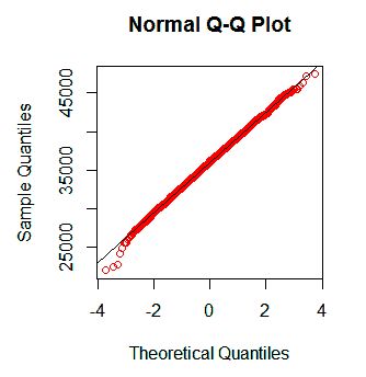
Another method to compare a sample against a Probability distribution is called the Q-Q plot, where when two distributions are similar then the plot will approximately lie on the line y = x and if they are linearly related then the plot will lie on a line but not necessarily on the line y = x. The Q-Q plot of our sample against the Normal distributions is:
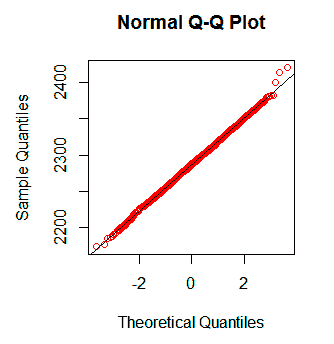
Q-Q plot of our sample data against the normal distribution. The sample data looks very normal as in the previous tests.
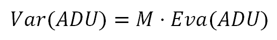
Once again, we have found the data consistent with the Poisson distribution with large mean, approximated to the Normal distribution. However, we have just used one patch from one shot. Nonetheless, there is a way where we can test in a more convincingly way that the photon noise follows a Poisson distribution: This distribution has the particular property that its mean (estimator of the Expected Value) is equal to its Variance.
It is customary to represent the Poisson distribution Mean and Variance them with the Greek letter lambda "λ", as we will do in the following equations: "λ" will represent the Expected Value and the Variance of the electron count in each photosite. As a count of elements, technically λ is dimensionless. Nonetheless, to make more understandable the equations, it is used with the fictional unit ADU when representing the Expected Value or Noise (Standard Deviation) and ADU² when the representing Variance.
If we evaluate the Expected Value to both equation sides of our model prototype we get:
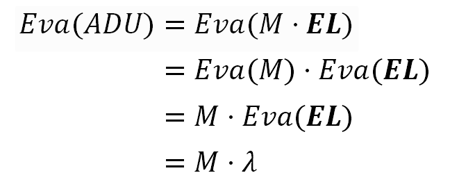
If we evaluate the Variance to both equation sides of our model prototype we get:
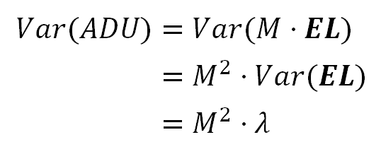
Now, if we replace "λ" in this last equation with the previous one in the Expected Value formula, we finally get:
Formula 2. The luminosity variance has a linear relationship with its mean value.
These last equations, derived from our model prototype, are all of them over-simplifications of the sensor noise model, disregarding other sources of noise that we will include later. Despite of that, they are still useful to show the Photon Noise as a fact has a Poisson distribution, because this source of noise is the main noise component in our data. We will develop more fitted equations later.
The formula 2 tells that under the assumption the noise has a Poisson distribution, the image luminosity Variance (the square of the noise) will have a linear relationship with its Expected Value.
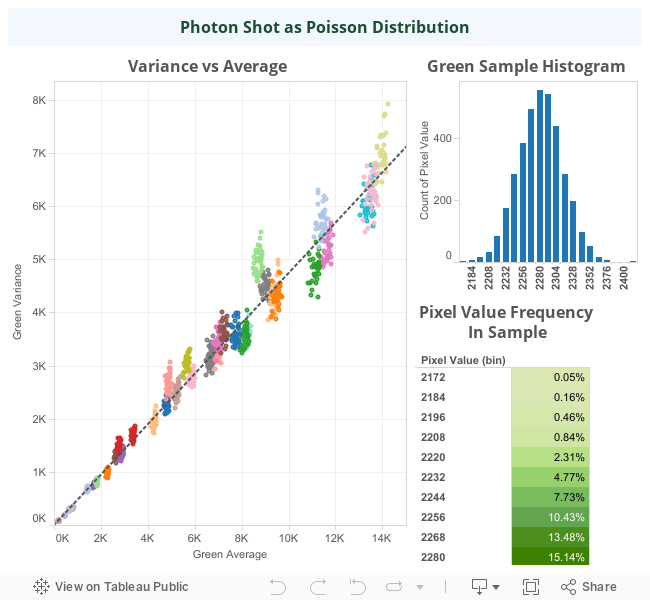
As estimators of the Variance and Expected Value we can use the sample average and variance from the 35 patches in the 34 raw image files of the chart we show before. To this effect, we have taken a square sample per patch (60 pixels per side) from the green raw image pixels and calculated the Variance and Average value from those 3,600 pixels per sample.
In the following image, we show the plot of each sample Variance (vertical axis) against it Average (horizontal axis), where the data from the same patch in the chart has the same color code. We can see there how they really have a linear relationship. In fact the dotted line trend shown in the plot, correlating the Variance with the Average, has a Coefficient of Determination (R²) of 99.3% and a p-value < 2.2E-16, as indicators that the linear model for the data is very significant, which in turn allows to say the Photon Noise has a Poisson Distribution with a chance virtually zero of being wrong.
The picture also shows the histogram of the sample for which we run successfully Normal distribution tests, there we can almost see the Gaussian bell shape. The pixel values in the histogram are in bins of 12 values.
If the Photon Noise were the only source of noise in the image, the SNR would be the square root of the average count of electrons collected (the square root of lambda "λ" in the following equations). Notice this is a limit imposed by a physical property of the light. A camera sensor noise can be assessed with respect to this limit knowing its SNR can not be better than that.
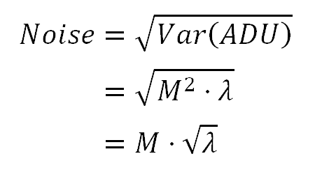
Formula 3. The Photon Shot Noise.
In the following equations, remember the noise is the square root of the Variance.
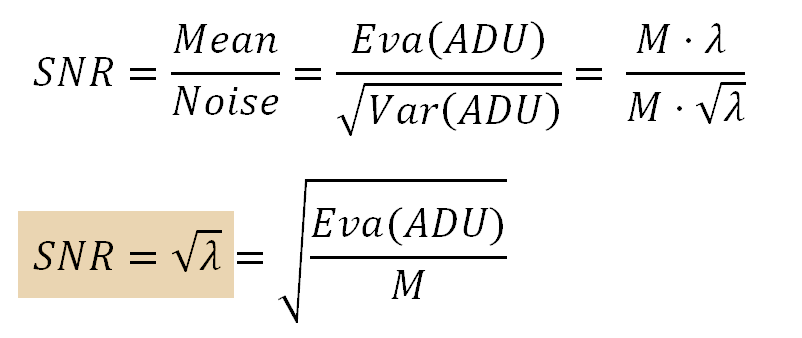
Formula 4. The Photon Shot SNR.
The last equation represents the SNR of an ideal camera sensor, where the only source of noise comes from the nature of light and there is not other source of noise.
When the SNR is expressed in logarithmic way, the Photon Shot Noise SNR gets represented as a line with slope of ½. If we take logarithms to both ends of the equation above, we get:
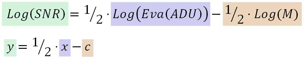
Formula 5. The logarithm of Photon Shot SNR and the logarithm of Average luminosity have a linear relationship with a slope of ½.
As summary, we can say about the Photon Shot Noise:
- Its proportional to the luminosity average square root. This means its Variance grows linearly with the luminosity (or signal).
- It has a Poisson distribution, which for luminosity above
1,000 ADUsis very similar to the Normal distribution. - Its SNR grows with the luminosity square root.
Read Noise
The following equation shows our current sensor model. As the "EL" term, representing the amount of electrons collected by the photosite, is a random variable we will show it using bold typeface.
In APS (from Active Pixel Sensor) sensors, each photosite is connected to the electronic circuitry in charge to convert the charge from the electrons —produced by the photon shots— to voltage, and conduct it as input to the A/D Converter. As this processing line is not perfect, the output of the A/D Converter is not exactly proportional to the amount of electrons from the photon shots. There is always a bias or base level of ADUs coming out from the A/D Converter, even when there are not electrons at all in the photosites, as in a photograph taken with lens cap on. This noise is called Read Noise and in summary it comes from the process of reading "how many" electrons are in the photosite and "calculating" the corresponding ADU value.
The following animation explains how the Read Noise base line is clipped from the ADU values, but even though the Read Noise stays in the image.
Simulation showing how the signal (2) gets mixed with the read noise (1), and how even after the read noise bias is removed (3 to 4) the resulting signal (4) still contains the read noise (3).
The sensor Read Noise. It is like "a fake signal" around an average of 500 ADU (in this example). The intensity of the noise in this graph is represented by the height of the emerald band.
The signal collected in the photosites. Even when the source is uniformly lit with an expected value of 300 ADU, the signal (red thin line) is not flat because it contains the Photon Noise.
The output of the A/D Converter, represented by the red thick line, contains the Read Noise and the signal. It contains more noise than the original signal in the step (2), because it also contains the Read Noise.
The Read Noise "correction". The Read Noise "fake signal" is subtracted from the ADU values. If the result of this subtraction is a negative value, the pixel is set to zero. Now the red signal has an average of 300 ADUs as expected, but the additional noise that came from the Read Noise is still there: the height of the emerald band is the same as in the step 3. This Read Noise correction, in some camera brands (e.g. Nikon) is made in-camera or otherwise by raw image processing software.
The following animation shows the same steps we saw above, but this time from the Histogram perspective.
Animation 2. Simulation of the histogram of signal mixed with the Read Noise and its clipping during its correction.
We will add the Read Noise to our model using the term "RNS", it represents the Read Noise "signal component" in each photosite ADU reading. It is in bold typeface because it is a random variable, it varies from photosite to photosite.
Formula 6. The Read Noise is added to the model.
To simplify our formulas, the term "RN" will represent the Read Noise, so "RN²" will represent its Variance:
Var(RNS) = RN²
StdDev(RNS) = RN
We will use the Linearity of Expectation property to get the Expected Value of the ADU values including the Read Noise. Applying the Expected Value operator to both ends of the equation above, we get:
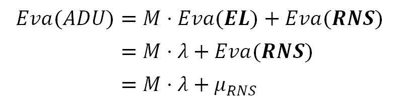
Formula 7a. Expected Value of the pixels considering the Read Noise.
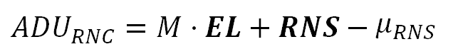
The formula above tells the average pixel value, in an image with Read Noise, is incremented by the average signal from that Read Noise. However, as we have already seen, this bias is removed in the "Read Noise correction". We will represent that correction in our model by subtracting the term μRNS:
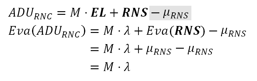
Formula 7b. Expected Value of the pixels after the Read Noise correction.
At the left side of the first equation above, the ADU term subscripted with "RNC", represents ADU values in a "Read Noise Corrected" raw image.
After the "Read Noise correction" the Read Noise "fake signal" is removed subtracting its average from the ADU values. This way, as we can see in the second equation above, the Expected value of the "Read Noise Corrected" raw image does not have the Read Noise "fake signal". Notice that RNS is a random variable but its average μRNS is a constant.
We must distinguish two different effects of the Read Noise: (i) It adds a bias to the photosite values and also (ii) increments their Variance. The Read noise correction removes the bias in the photosites values, but even though, the added Variance stays in the image.
This is represented in the animation with the height of the emerald band: the signal noise in the stage (2) is incremented by the Read Noise in the stage (3) and remains that way even after the Read Noise correction in (4).
We are interested in the noise in the raw image file we will process to get our final image, and that will be the raw image after Read Noise correction. For this reason, from now on, we will keep using as model, the formula with the Read Noise "fake signal" removed.
It must be clear the Read Noise is completely independent of the Photon Noise. The Read Noise is related to imperfections in the sensor electronic and is independent of the intensity of the light hitting the sensor. On the contrary, the Photon Noise is caused by the physical nature of the light and related to its intensity but is totally unrelated to the sensor processing.
This independence between the Read and Photon Noise means the Variance of their sum is equal to the sum of their Variances.
We get the variance in the model applying the Variance operator to both ends of the equation above. The Variance of a non random variable as μRNS is zero.
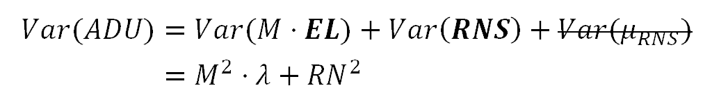
Formula 8a. Variance of the model with Read Noise.
Now we can get the SNR in our current model. Remember the noise is the square root of the Variance, which is the Standard Deviation.
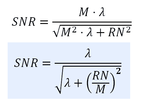
Formula 8b. The SNR in a sensor with only Read Noise and Photon Shot Noise.
If we compare the SNR of this sensor model —with Photon Shot and Read noise— against the ideal sensor, we get the behavior shown in the following graph. In that graph, the values themselves are not relevant, it is just a simulated example.
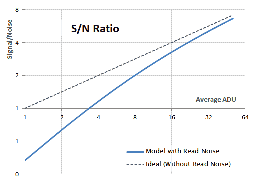
log-log graphic comparing the SNR of a sensor with Read and Photon Shot noise (blue curve) against an 'ideal' sensor with only Photon Shot Noise (gray dashed line).
Notice how the Read Noise hurts the darker parts of the image diminishing the SNR. For greater levels of luminosity, the effect of the the Read Noise fades away and the SNR gets asymptotically closer to the ideal SNR sensor.
It is said the Read Noise imposes a lower limit to the sensor range, we will see why. Lets suppose we won't tolerate a SNR below 2 (yes, this is an awfully low value, but this is just an example to get the idea). In the ideal sensor (dotted line), this would require expositions bringing luminosity values above or equal to 4 ADUs. However, in the sensor with Read Noise, this requires expositions with ADU values above or equal to 8 ADUs, this is 1 stop more! This means the Read Noise has reduced the camera dynamic range for 1 stop: to avoid non tolerated levels of noise we can't use one more stop in the sensor output range.
In some camera brands, an exposure with the fastest shutter speed and the lens caps on, brings a raw image with only the Read Noise (called a "Black frame"), corresponding to the stage 3 in our previous animations. In that case the processing of the raw image must remove the Read Noise.
Nikon cameras bring raw images with the Read Noise already corrected, corresponding to the stage 4 in our animations. In this case, the raw image values are represented by our last model formula. In the case of Canon cameras, the raw image processing software must do the Read Noise correction.
Most Nikon cameras include, in the raw image file, data from the sensor area containing the "Optical Black" (OB) photosites. These photosites have a dark shield covering them, so the light can not hit them. They are useful to find out the Read Noise signal level.
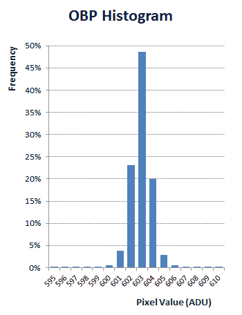
Histogram of the pixel values from the Optical Black area in a raw image file from a Nikon D7000 camera (ISO 100).
The sensor uses this data to make the in-camera "Read Noise Correction". The histogram above corresponds to real data from the pixels in the OB area in a raw image file from a Nikon D7000 camera using ISO 100. This corresponds to the histogram in the stage 1 in our above animations.
In the histogram profile, the 96% of the pixels have a value equal or below to 604 ADU. We can get a clue about how this value is used for the in-camera "Read Noise Correction" by watching the upper values in the histogram of a severely over-exposed image as in the following picture.
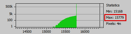
Upper side of the histogram of an overexposed image.
The histogram above corresponds to real raw data from an overexposed shot taken with a Nikon D7000 also using ISO 100. Notice how the green pixels overflowing 16,383 ADU, which is the top limit in 14-bit raw files, were clipped to that maximum value in the stage 3 (in our animations above).
In the stage 4, the 604 ADU value —selected from the OB pixels— was used by the sensor to "Read Noise correct" the image, resulting in 16,383 - 604 = 15,779 ADU which is the top value we see in the final histogram above.
After this correction, only the 4% = 100% - 96% of the Read Noise "signal" still remains in the image values. But besides of being a low percentage, they are —at most— values around 7 ADUs (the remaining Read Noise values over the subtracted 604) added to image.
PRNU Noise
All the photosites are not made equal —even those filtering the light for the same color— are not perfectly equally sensitive to the light. The micro-lenses over each photosite, the layer collecting the produced electrons, the A/D converter and other sensor circuitry elements are not all manufactured perfectly equal to each other. In other words the "M" term in our model, is not exactly the same value for each photosite. Instead, "M" is an attribute of each photosite. This condition is called Pixel Response Non-Uniformity (PRNU).
Considering this, we will replace the factor "M" with "Mp": we will use the subscript "p" as indication that "M" varies for each photosite on each given sensor position "p".
Formula 9. Adding PRNU to the sensor model.
We must notice the sensitivity variations of "Mp" are not intended, they are random changes from photosite to photosite. In this sense, "Mp" is a random variable with respect to the surface of the sensor. This fact is represented in the notation —of the formula above— with the use of bold typeface for "Mp". However, we will consider that each photosite, along the time, has always its same "Mp" value. This means "Mp", for each photosite, is a constant along the time (between shots) when keeping the same ISO speed (the photosite sensitivity changes with the ISO speed).
The average value (statistically speaking, the Expected Value) of all the "Mp" factors, corresponding to all the photosites in the sensor surface, is a constant. This average is probably what the manufacturing processing was aiming for. We will call "EM" (for Expected Multiplier) to this average:
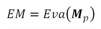
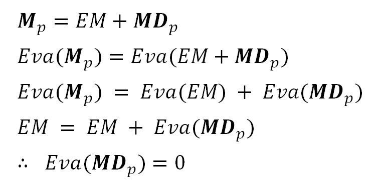
We will model "Mp" as variations around this average. To this effect, we will consider "Mp" as composed by two additive components (this is plausible considering this formula for the Eva() of the sum of two variables): one is the average "EM" and the other is the photosite sensitivity deviation with respect to that average. We will call "MDp" to this latter component (for "M" Deviation):
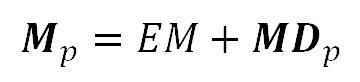
Notice that this way to express "Mp" implies that the average of "MDp" is zero ( Eva(MDp) = 0 ). We can probe this applying the Expected Value operator to both ends of the previous equation and using "Eva(EM) = EM" (justified by this formula for the Eva() of a constant):
Updating our sensor model in the formula 9 with our above definition of "Mp", we get:
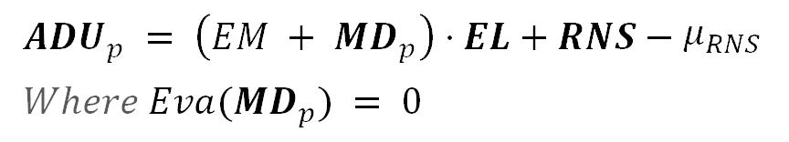
Formula 10. Sensor model considering PRNU, Read Noise and Photon Shot noise.
The three sources of noise, represented with bold typeface, are independent of each other. This will allow us to use simpler formulas to get the Expected Value and the Variance of the resulting ADU.
The Spatial Average ADU value
To get the Expected Value of the sensor photosite (estimated by their mean value) in our model, we will apply the Expected Value operator to both ends of our model equation. We will also use this equation for the Expected Value of a product of independent variables, among other ones we have already used, to get:
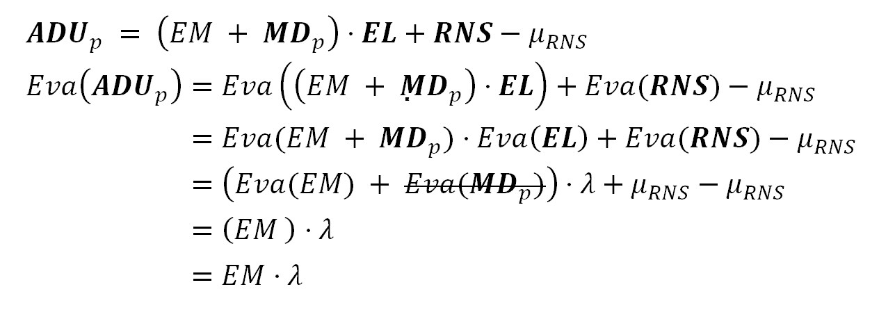
Formula 11. Expected Value in the sensor model.
The Spatial ADU value Variance
To get the (spatial) Variance —in our model— we will use this equation for the Variance of a product of independent variables among other ones we have already used. At the beginning, we get these equations, where the terms with value zero are shown stricken-through.
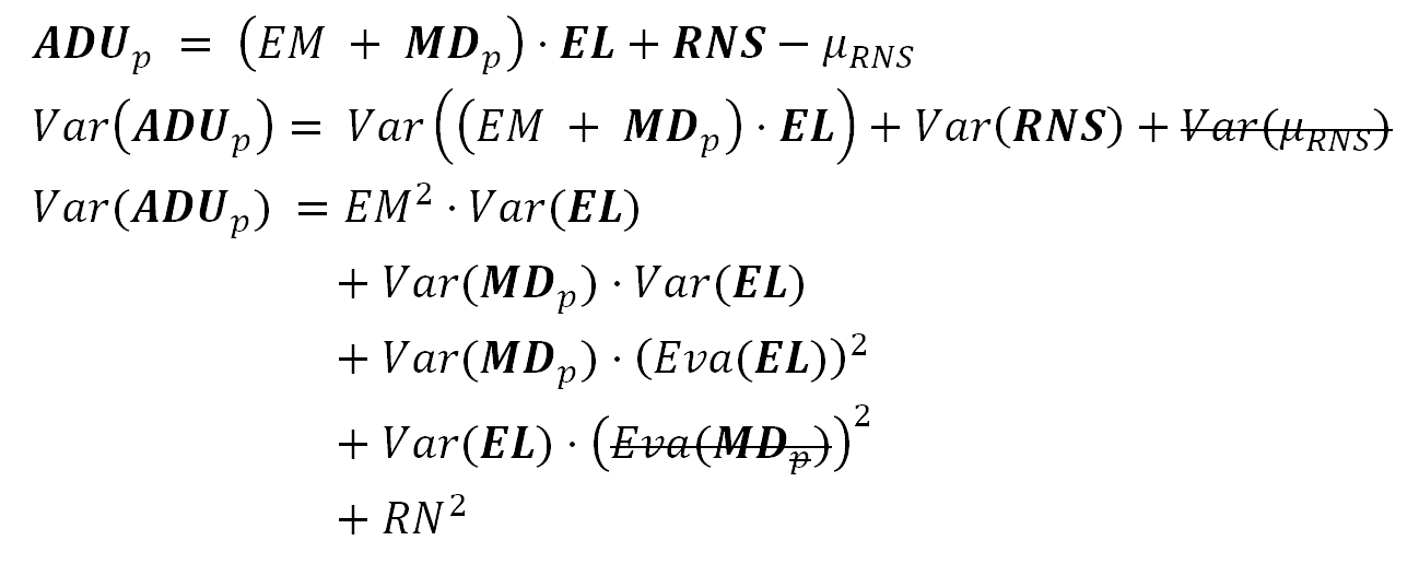
Variance in the sensor model. Initial equations.
As a matter of notation, we will refer to the Variance of "MDp" as "PRNU²". This way the term for the PRNU noise is "PRNU".
Please notice the equation symbol "PRNU" refers to the Standard Deviation of the photosites sensitivities (in ADU/e-) and not to the noise this PRNU will cause in the raw image (in ADUs).
Var(MDp) == PRNU²
StdDev(MDp) == PRNU
Also we will use the following equations, already explained:
Var(EL) = λ
Eva(EL) = λ
Eva(MDp) = 0
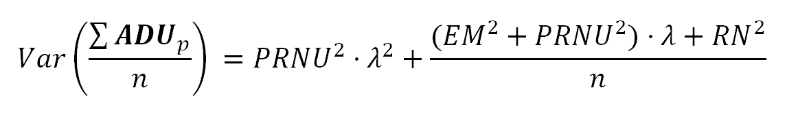
The resulting Variance is:
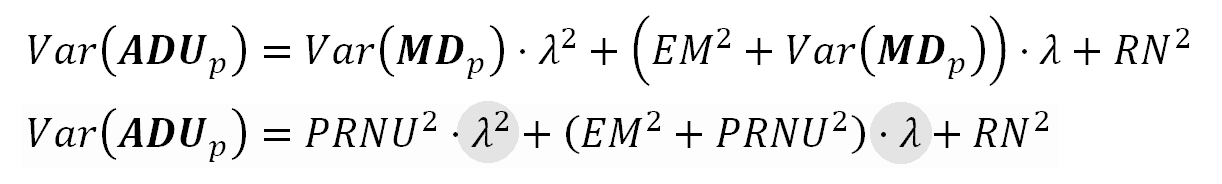
Formula 12. Variance in the sensor model considering PRNU, Photon Shot and Read noise.
This is the equation we were looking for from the beginning of this post. A simple equation aroused from the sensor model explaining the noise profile, right from the sensor characteristics.
Notice how the Variance is a quadratic polynomial of λ, which represents the average count of electrons in the photosites. The quadratic term is the synergy between the PRNU Noise and the Photon Noise. Besides of the quadratic term, the PRNU also has impact in the linear λ term, all of this tells us the variance of sensitivities among the photosites (PRNU) can be a very strong source of noise.
The noise (Standard Deviation) is just the square root of the variance in the above formula 12. This way, the SNR is:
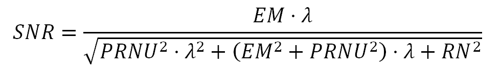
Formula 13. SNR considering PRNU, Read and Photon Shot noise.
The PRNU SNR Limit
If the PRNU were the only source of noise in the sensor, the total ADU Variance would be mainly the quadratic term of the Variance we found above. In such case the SNR would be:
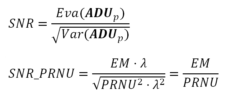
Formula 14. SNR limit caused by PRNU noise.
Notice how this SNR is independent of the electron count. This is also the SNR top limit when we consider all the three noise types as in the formula 13. More formally: if the value of λ in the formula 13 keeps growing, the resulting SNR will always stay below the SNR_PRNU value we have found in the above.
Fortunately, for most DSLR camera sensors, the PRNU noise starts kicking close to the top limit of λ (e.g. 16,383 ADU for 14-bit raw files) and do not cause too much damage to the SNR just because the λ range ends before.
The Three Noise phases in the SNR
In the following graph we have a simulated SNR curve, where we can distinguish three phases showing the dominance of each noise type we have studied. At the left end of the curve, with low ADU values —in the area shown with orange background— the Read Noise makes the SNR somewhat below to the gray dotted line representing the ideal sensor, with only Photon Noise. In the second part, shown with green background, the SNR is dominated by the Photon Noise and "stays" with a slope around 0.5. At the right end —in the area shown with pink background— the SNR slows down its growing rate and starts to bend over, to stay asymptotically below the PRNU limit (see formula 14), shown with a dotted red line.
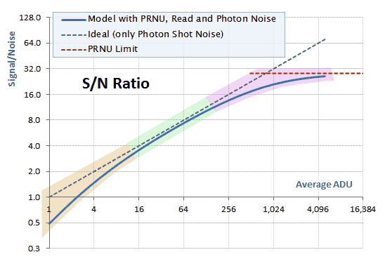
SNR phases. Orange: Read Noise, Green: Photon Shot noise, Red: PRNU noise
Isolating the Image PRNU Noise
We can isolate the image PRNU noise by averaging a set of identical shots of a uniformly lit surface —slightly out of focus— and with rather over-exposure settings, but taking care to do not get highlight clipped values in the raw image. This way we will make a greater presence of the PRNU noise on each image. Notice this averaging is not as before, over the image surface, but over the same pixel —each one of them— which is averaged over a set of shots.
Notice here we are talking about the noise in the image (in ADUs) caused by the non constant photosites sensitivities (PRNU). To emphasize that, we are using the expression "image PRNU Noise". Please, don't get confused with the symbol "PRNU" in the equations, which represents the Standard Deviation of the sensor photosite sensitivities (in ADU/e-).
The image averaging will make stand out the PRNU noise, because —for a given pixel— it doesn't change from shot to shot. However, the other types of noise (Photon Shot and Read), randomly changing from shot to shot, will diminish in the average. We will see this more clearly from the following formulas.
The next equation models the image averaging.
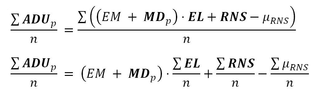
Formula 15. The average of the same pixel between images.
In these formulas, as we are averaging the same pixel in a set of raw images, the sums are done for each fixed "p" subscript. That is the reason why we can factor "MDp" out of the sum in the first equation. The number of averaged images is represented by "n".
If we apply the Variance operator over both ends of the last equation above, we will get:
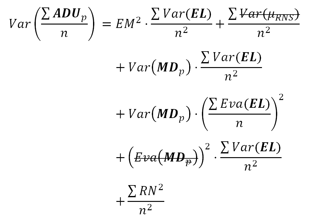
Formula 16. Variance of the average of the same pixel between images. Intermediate equation.
At the end we will get the following equation.
Formula 17. Variance of the average of the same pixel between images.
In the above equation we can see how the PRNU quadratic term is not affected by the averaging, while the impact of the other kinds of noise diminishes with greater "n" values, the number of averaged images.
We have taken 32 shots with the camera lens standing over an iPad screen showing a monochromatic image. The resulting raw images have green pixel values at the 87% of their top limit. In other words, they are overexposed but not overflowing their top limit.
To show the effect of this averaging over the Variance of the resulting image, the following graph shows the plot of each individual image green photosite noise (Standard Deviation) and also the noise from the image resulting from the average of a different number of photographs. We got those average images using Iris software (add_mean command).
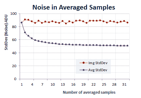
Noise decreasing with the number of averaged samples.
Each photograph contains additional Variance coming not by noise but for the lens vignetting. For this reason the graph above shows data from a 46 by 66 pixels sample area, chosen for being a uniformly lit image area.
The noise of the average image decreases very marginally from around 20 samples. However, we have averaged all of them, resulting the following image. A tone curve was applied to make more easier to see the lens vignetting.

Average image with undesired vignetting.
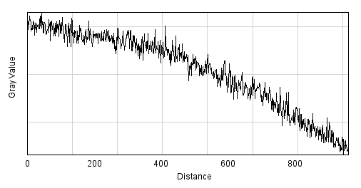
If we draw a line from the center of the image to one of its corners, and plot the pixel values along that line, we will get the curve shown in the following graph, where the high frequency (spatial) changes in pixel values are caused —mainly— by the PRNU noise. The vignetting is the cause of the overall trend curve with the arc shape.
To isolate the image PRNU noise from the lens vignetting, we have get rid of that arc shape and get the PRNU noise "over" a flat line.
One way to remove that lens vignetting is using a technique called Flat-field correction. In the general case, the flat field correction requires the subtraction of a "dark frame" to remove the Read Noise and possibly other kinds of sensor noise (e.g. thermal noise). However, for the Nikon camera —as we have already seen— the raw image file comes with this correction already done for the Read Noise and neither we have the thermal noise that arises from multi-second expositions nor we have considering it in this article.
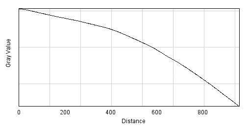
First, we will de-noise the average image, applying some Photoshop filters (strong Noise reduction and some Gaussian Blur) in order to remove the high frequency changes and get only the background with the lens vignetting, we will call "flat field" to that resulting image.
To make the Flat-Field correction, we divide each pixel value in the averaged image by the corresponding one (with the same position coordinates in the sensor) in the flat field image (pixel by pixel, using ImageJ software) and then we multiply the result by the median pixel value in that flat field.
pixel(prnu_only, x, y) = [pixel(averaged_image, x, y)/pixel(flat_field, x, y)] * median(flat_field)

    Where pixel(img, x, y) is a function allowing to get or set the value
    of the pixel with coordinates (x,y) in the image file "img".
The resulting isolated image PRNU noise is shown in the following image. That image has been processed to make more evident its structure. The top half shows the image PRNU noise at 100% scale; there is a (bad cleaning) smudge in the bottom left side. The bottom half shows another part of the image PRNU noise but at 50% scale, it makes more apparent a vertical pattern, but also shows there is some horizontal pattern.

Nikon D7000 PRNU at ISO 100. The top clip is at 100% scale and the bottom at 50%. In both cases a vertical pattern is apparent. In the bottom clip also a slight horizontal pattern can be noticed.
As we can see, the PRNU noise in the spatial dimension is not totally random, it can probably be decomposed in three parts: column, row and a remaining random spatial components. Setting aside what we just said, the analysis of a sample of the PRNU noise shows it has a distribution very close to the Normal one:
> shapiro.test(prnu$PixelValue)
"Shapiro-Wilk normality test"
W = 0.9993, p-value = 0.03502

> ad.test(prnu$PixelValue)
"Anderson-Darling normality test"
A = 0.5389, p-value = 0.167
The sample rejects the normality hypothesis in the Shapiro-Wilk test but fails to reject it in the Anderson-Darling one, and its Q-Q plot against the Normal distribution is not too bad at all as is shown in the following picture.
Q-Q plot of PRNU noise against the Normal distribution.
Removing (most of) the PRNU Image Noise
One way to remove most of the PRNU image noise is taking the difference —pixel by pixel— of two identical images: we take two identical photographs with identical scene, illumination, and camera settings: like two consecutive images of a still target in a shooting burst. Please notice that in our nomenclature, the term PRNU is the Standard Deviation of the photosites sensitivities, which in turn causes noise in the image called PRNU image noise.
The idea is that being the PRNU caused by a term (MDp) which remains constant between identical shots, we will be able to removed it in the difference of those two images.
Lets see the idea through the equations in our model. We will use the delta "Δ" operator to denote the difference of the values from the same pixel in two identical shots. The delta of μRNS, as the delta of a constant value, is zero.
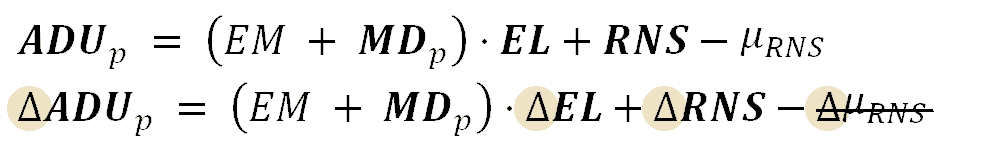
Formula 18. The difference of values of the same pixel in two images.
As "MDp" is a photosite characteristic and doesn't change between shots, we can factor the term out of the delta operator.
Now we apply the (spatial) Variance operator to both sides of the last equation. Eventually we will get the following one:
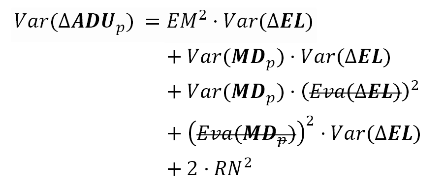
The (spatial) Variance of the difference of values of the same pixel in two images.
The stricken-through terms have zero value. At the end, we will get the following equation.
Formula 19. The (spatial) Variance of the difference of values of the same pixel in two images.
Notice the right side of above equation is similar to the ADUp Variance formula 12 but —as we wanted— it does not include the quadratic term of the PRNU variance! Even when it includes the PRNU linear term (in "λ"), the PRNU variance (PRNU²) is usually very much smaller than the "EM²" term. As a practical consequence of this we can disregard the PRNU² term and consider the result contains only Read and Photon shot noise.
The formula 19 tells that if we compute the image difference between two identical shots, and divide it by the square root of 2, the resulting image will contain —mostly— only the Photon and Read Noise in the original images (the ones used to compute that difference image).
An example (of the difference image divided by the root square of 2) is shown in the following image.

Nikon D7000 Photon and Read Noise at 100% scale. Image processed to make its structure more apparent.
Further analysis will show the Read Noise is relatively very small and the above image contains almost only Photon Shot noise, which —as expected— does not contain any pattern, is is almost just Gaussian noise.
Summary of Formulas Modeling the Sensor Noise
We have developed few formulas modeling the image raw pixel value and its statistics. During that development we have shown many intermediate equations explaining in detail how we got the final main equations. Here we will summarize the main equations we will use in future camera noise analysis articles.
The Raw Image Pixel Value
The pixel value in a raw image file can be described as:
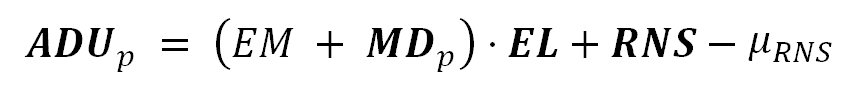
Formula S1. Raw image pixel value, from the sensor photosite, in ADUs.
Where "EM" is the average ratio used by the sensor to convert the electron count in each photosite to pixel value units (ADU). The "MDp" term represents the photosite sensitivity deviations around their media value "EM", and the sum of these both terms is the ratio used for the photosite for the conversion of its electron count to ADU units. The count of electrons in the photosite is represented by "EL".
The "EM" and "MDp" terms are given in "ADU/e-" units, while "EL" is in "e-" (electrons) units. This way the product result is in "ADUs".
The term "RNS" is the Read Noise "fake signal" bias added by the sensor circuitry to the "real signal", and is given in ADU units. The term μRNS —also given in ADUs— is the average value of that Read Noise "fake signal" bias, which is subtracted from the photosite reading to remove it.
We must distinguish two different effects of the Read Noise: (i) It adds a bias to the photosite values and also (ii) increments their Variance. The Read noise correction removes the bias in the photosites values, but even though, the added Variance stays in the image.
The following equation describes the Expected Value of the sensor photosite reading from an image area, corresponding to a uniformly lit surface causing the same flux of electrons on each photosite. Here we are assuming there is not light fall off caused by —for example— lens vignetting. The same context will apply to the Variance formula we will show below.
We will estimate this Expected Value through the arithmetic mean of the raw image pixel values.
Formula S2. Expected Value of the pixel values.
In the above equation, "λ" represents the Expected Value of the electron count in the photosites.
The Raw Image Pixel Value Variance
The following formula models the Variance of the sensor photosites readings from an image area corresponding to a uniformly lit surface. As the count of electrons in each photosite —after a photograph exposition— follows a Poisson distribution, their variance and their Expected Value have the same λ value.
We need the (spatial) Variance to measure the noise. The noise is measured by the Variance square root: the Standard Deviation statistic of the raw image pixel values.

Formula S3. Variance of the pixel values.
In the equation above, the term "PRNU²" is the variance of the sensor photosites sensitivities, this is the variance of "MDp" in the formula S1. Do not confuse it with the image PRNU noise this will cause. The term "RN²" corresponds to the Read Noise variance, which is just the square of the Read Noise measure.
The Variance of the Difference of two Identical Images
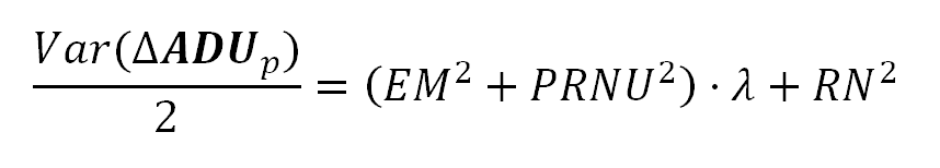
We can measure the sensor noise, with the PRNU noise component removed, by using the following equation.
Formula S4. Variance of the difference of two images.
This equation models the Variance of the difference of two identical images: Two identical photographs of the same scene, with identical camera settings and illumination: like two consecutive images of a still target in a shooting burst.
If we take two identical photographs to the same uniformly lit surface, and we subtract each pixel value in one image from the corresponding pixel —the one with the same position in the sensor— in the other, the half of the pixel values Variance in the resulting image will be equal to the right side of the equation above: the linear part of the equation in the formula S3.