In the article "Developing a RAW photo file 'by hand'" we learned many photograph concepts and how to handle and develop, by ourselves, a raw photo file (without demosaicing). However, an important part of the development process was done using IRIS software, which is a Windows only (free) product, which restricted users of other OSs to repeat the article exercises.
Furthermore, the application of tonal curves has to be done using Photoshop, which automatically makes additional image changes when applying a curve, like hue and saturation adjustment for a better looking image or for film-like results. That is a not at all a 'by hand' DIY kind of tool we wanted to use, but we didn't had any other choice.
To overcome this, and many other difficulties, we have developed the imgnoiser R Package, and now all the Development of a RAW Photo by hand can be done using that and other R packages.
An additional and great benefit of the photograph development in the R environment, is that you can code your own ideas and make more experiments with the image in a completely impossible way for the environment we used in the original article. As usual, we will include all the required R code to reproduce all the described exercises.
In this post we will explain again the Raw Development by hand but focused in the operational part using R tools, and in new topics, but without explaining the photograph concepts we have already learn in the original post. Also, we wont explain in detail the usage of the imgnoiser package; you can learn about that topic reading the article Introducing the imgnoiser R package.
The Required Software
Besides the imgnoiser and the standard R Packages, we will use also the following packages:
tiffRead and write TIFF imagesggplot2An implementation of the Grammar of GraphicspixmapBitmap Images ("Pixel Maps")gridThe Grid Graphics Package
I use R Studio as IDE for R.
We will extract the photosite readings from the raw image using dcraw, which is free open source software with available binaries in the web for all the main OSs.
Getting the Raw Channels Data
We will extract the raw data as a linear grayscale image using the following command line:
dcraw -D -4 _ODL9241.NEF
Where the -D option is for original unscaled pixel values and -4 is to get linear 16-bit values. The file name _ODL9241.NEF is a photograph from my Nikon D7000 camera; this is the same image we used in the original post.
The output from the above command is a .pgm file with the same base name as your raw file name; in my case it is _ODL2240.pgm.
Now, in R, you can read and split the four channels in the gray-scale .pgm image with the split_channels() function.
img.chs <- imgnoiser::split_channels('_ODL9241.pgm')
str(img.chs)
#>  $ ch1: int [1:1640, 1:2474] 1095 1018 998 1006 1041 1027 1028 1025 1061 1068 ...
#>  $ ch2: int [1:1640, 1:2474] 2023 1986 2025 1973 1949 1993 1981 2026 1998 1965 ...
#>  $ ch3: int [1:1640, 1:2474] 2015 2018 2010 2001 2015 1988 2009 2003 2046 2005 ...
#>  $ ch4: int [1:1640, 1:2474] 1356 1317 1318 1345 1320 1312 1348 1320 1340 1267 ...

class(img.chs$ch1)
#> [1] "matrix"
This way we get a list of matrices (named ch1, ch2, and so on) with the channels in raw image. You should know, which correspond for each color filter in your sensor photosites. For Nikon cameras they are RGGB.
The matrices resulting from the split_channels() function contain in the position [1,1] the image top left corner and in [nrow(img$ch1), ncol(img$ch1)] the bottom right image corner, where —as you may have noticed— the rows corresponds to the y axis and the the columns to x one.
You can use the graphics::image function to display the image. However, that function plots the matrix rows in the x axis (horizontally). To display correctly our image channels we have to sync our columns and rows as they want, using the following code:
image(t(img.chs$ch2[nrow(img.chs$ch2):1,]), col=gray((0:255)/255), axes = FALSE, useRaster=TRUE)
We can also use the pixmap::pixmapGrey() function to display a channel. This function expects values in the [0, 1] range. As the maximum possible value in our raw photo is 16284 we will divide the image pixel values by this number to comply with the expected range.
pm <- pixmap::pixmapGrey(img.chs$ch2/16384)
plot(pm)
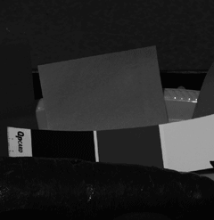
The channel #2 in our sensor corresponds to one of the green channels. Using the function above, it looks like this:
If you want, you can save each of your image channels as .tif grayscale images using:
tiff::writeTIFF(img.chs$ch1/16384, '_ODL9241_red.tif', bits.per.sample = 16)
tiff::writeTIFF(img.chs$ch2/16384, '_ODL9241_green.tif', bits.per.sample = 16)
tiff::writeTIFF(img.chs$ch4/16384, '_ODL9241_blue.tif', bits.per.sample = 16)
Each pixel value in each channel is divided by 16384 because the writeTIFF function expects tone values in the [0, 1] range.
White Balance
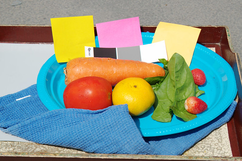
We need to white balance the image. Fortunately, our image contains a strip of neutral patches to help us to do that. If that is not your case you need a shot with the same lighting environment with an object with neutral color.
To white-balance the image, we need the average raw pixel values in the neutral patch. For that matter, we will use the middle gray patch in the image. To get those average pixel values, we can use the image displayed above to locate a window containing only the gray the patch pixels.
As first a approach, eyeballed from the above image, we will check in a window containing the top half and +/- 400 pixels around the horizontal image center:
pm <- pixmap::pixmapGrey(img.chs$ch2[1:820, 837:1637]/16384)
plot(pm)
Navigating this way in the image we can locate the gray patch in [522:582, 1252:1400]. Nonetheless, you can make your life easier just opening the image using regular software and looking for the gray patch window coordinates. Also you can use rawdigger to directly select an area in the gray patch and get the neutral raw reference values. Just remember the raw channels are a half of the image developed with regular software (demosaiced).
Now we can crop a window containing only the gray patch pixels, and get the mean pixel value on each channel:
# Crop the gray area
gray.crop <- lapply(img.chs, function(img) img[522:582, 1252:1400])
# Compute the mean channel values
lapply(gray.crop, mean)
#> $ch1
#> [1] 1523.553
#>
#> $ch2
#> [1] 2997.766
#>
#> $ch3
#> [1] 3005.152
#>
#> $ch4
#> [1] 2128.173
The mean channel values, we will use as neutral reference, are (1523.5, 2997.8, 3005.2, 2128.2) (in RGGB). We will average both green average pixel values to get a simple RGB neutral reference as required by imgnoiser, to obtain (1523.5, 3001.5, 2128.2).
Color Space Conversion
Now we will create cm, an instance of the imgnoiser::colmap class, with the camera color data corresponding to the Nikon D7000, which is the camera we used to take the photograph we are developing. Then, we will ask to this cm object to get the calibration for our neutral reference color, for the conversion to the sRGB space.
# Create cm
cm <- imgnoiser::colmap$new(nikon.d7000.ISO100.colmap)
# Our gray patch neutral reference
neutral.raw <- c(1523.5, 3001.5, 2128.2)
# Compute the conversion matrix for the light causing this neutral values
mtx <- cm$get.conv.matrix.from.raw(neutral.raw, 'sRGB')
#> White Balance CCT:5034.92303729799
#> White Balance xy (1931):c(0.344636266858525, 0.356073278333864)
# Print the conversion matrix
mtx
#>             [,1]       [,2]       [,3]
#> [1,]  3.43183982 -0.6585254 -0.1176318
#> [2,] -0.35107805  1.6433204 -0.6559810
#> [3,]  0.03294311 -0.5018324  2.0945217
The get.conv.matrix.from.raw() function prints the CCT (Correlated Color Temperature) and the xy coordinates corresponding to the white point for our neutral reference. Also, this function returns the color conversion matrix from the camera raw space pixel values to the destination space, in this case sRGB. This matrix expects and produces RGB color components in[0, 1]`.
We will prepare and then use the cm object we just created to make the color space conversion. For the preparation we will call its prepare.to.dest.conversions() function. In that call we may define the destination scale, which by default is 255. Nonetheless, notice the conversion is made using floating point numbers. Also the result will be expressed with floating point values. This means, this destination scale does not have impact in the accuracy of the resulting image; we can change it any time later. This time we will use 16384 to stay in the same range containing the camera raw values.
The camera color data used in the creation of cm may contain a tonal curve (TC) prescribed for that particular camera. The use.camera.tc parameter allows to specify if we really want this TC applied to the resulting image or not; the default parameter value is TRUE. As for experience, we know this curve brings nice results, this time, we will apply it to the image.
With the conv.tone.curve parameter, we can also confirm if we want to apply the TC prescribed by the color space —in this case sRGB— the default value of this parameter is target.space.tc which means "apply the tone curve corresponding to the destination space". However, we can choose (linear, sRGB, ProPhoto, BT.709, Gamma.2.2, Gamma.1.8) and experiment mixing color spaces and tonal curves. This time we will just use the sRGB tonal curve.
As we said before, you should know to which photosite color filter correspond each channel we got using the imgnoiser::split_channels() function at the very beginning. The prepare.to.dest.conversions() function has the RGGB.indices parameter to specify that. This parameter default value is c(1,2,3,4), meaning that the first channel is Red, the second is Green and so on like in the RGGB sequence, which for most Nikon cameras is OK.
If that is not the channel sequence for your camera, and for example it is GBRG, the corresponding sequence looking for the RGGB channels is c(3,4,1,2) which is the value you should use as RGGB.indices argument.
cm$prepare.to.dest.conversions(
  dest.scale = 16384,
  use.camera.tc = TRUE,
  conv.tone.curve = 'sRGB'
  )

# Convert the raw image
rgb <- cm$convert.raw.to.dest(img.chs)
str(rgb)
#> List of 3
#>  $ r: num [1:1640, 1:2474] 10314 9798 9657 9725 9967 ...
#>  $ g: num [1:1640, 1:2474] 9857 9977 9963 9890 9946 ...
#>  $ b: num [1:1640, 1:2474] 9456 9292 9245 9454 9357 ...
Saving the Final Image
Now we can save the resulting image in a .tif 16-bit file using the tiff::writeTIFF() function, which expects an array with three layers (matrices) containing each of the RGB channels. As what we have from the convert.raw.to.dest() function is a list of those three matrices, we have to reshape our data before save it the tiff::writeTIFF() function.
# Prepare to save
raw.img <- array(c(rgb$r, rgb$g, rgb$b), dim=c(dim(rgb$r)[1], dim(rgb$r)[2], 3))
raw.img <- raw.img / 16384
# Save as tiff
tiff::writeTIFF(raw.img, '_ODL9241_sRGB.tif', bits.per.sample = 16)
We have just created a .tif image file in the sRGB color space (or profile), but this file doesn't have a tag indicating this fact. As consequence, some software may not display the image correctly. To fix this we can use —for example— Photoshop which may alert us —depending on your color settings— the file doesn't have a color profile and let us assign it one; in that case we have to assign it the sRGB IEC61966-2.1 color profile.
The resulting image from the previous steps (without any additional retouching) is:
Trying other Conversion Options
Without Camera Tone Curve
We can try again the conversion, but this time without the camera TC:
cm$prepare.to.dest.conversions(
  dest.scale = 16384,
  use.camera.tc = FALSE, # <== Without camera TC
  conv.tone.curve = 'sRGB'
)
# Convert the raw image
rgb <- cm$convert.raw.to.dest(img.chs)
rgb.img <- rgb(rgb$r, rgb$g, rgb$b, maxColorValue =16384)
# Prepare to save
raw.img <- array(c(rgb$r, rgb$g, rgb$b), dim=c(dim(rgb$r)[1], dim(rgb$r)[2], 3))
raw.img <- raw.img / 16384
# Save as tiff
tiff::writeTIFF(raw.img, '_ODL9241_nocam_sRGB.tif', bits.per.sample = 16)
This time we obtain:
Without the camera TC, the image is a little dark with lack of contrast.
Trying our own Conversion Matrix
We can test a color conversion matrix, not computed from the camera color data provided in the creation of the cm (colmap class instance), as we have been doing in the previous examples.
For example, lets try the conversion matrix published by DxOMark in the Color Response tab of each camera review. Which for my Nikon D7000 are:
#-- Using DxOMark matrices
d50.mtx <- matrix(c( 1.87,  -0.81, -0.06,
                    -0.16,   1.55, -0.39,
                     0.05,  -0.47,  1.42), 3, 3, byrow = TRUE)

a.mtx <- matrix(c( 1.82,  -0.74, -0.07,
                  -0.22,   1.52, -0.3,
                   0.07,  -0.63,  1.57), 3, 3, byrow = TRUE)
From the output of the get.conv.matrix.from.raw() function in previous examples, we can see our neutral reference corresponds to a CCT of 5035°K.
The matrices from DxOMark are for the D50 and A illuminants, corresponding to a CCT of 5000°K and 2856°K correspondingly. We might interpolate between those matrices looking for the matrix for 5035°K using the interp.matrix.by.inv.temp() function in the imgnoiser package. However, we can't because 5035°K is not in [5000, 2856]°K ; that would be extrapolating the DxOMark matrices, Which is not allowed by interp.matrix.by.inv.temp() because it is not recommended to do that:
mtx <- imgnoiser::interp.matrix.by.inv.temp(5035, d50.mtx, 5000, a.mtx, 2856)
#> Error in interp.matrix.by.inv.temp(5035, d50.mtx, 5000, a.mtx, 2856) :
#>   The 'cct.k' argument value must be between the illuminants CCTs.
Nonetheless, the 5035°K CCT for our neutral reference is very close to the 5000°K CCT of the D50 matrix. In general, CCT differences around 50/75 °K are not significant in the sense they render images with barely noticeable differences. So —fortunately— we can use the DxOMark D50 matrix without compromising the accuracy of the colors in the resulting image.
To plug in the the cm object the color matrix we want to use, we should use its set.conv.matrix.from.raw() function, instead of the get.conv.matrix.from.raw(), which is the function we have used in other examples.
We will call the set.conv.matrix.from.raw() function, using as parameters, the neutral reference and the matrix we want to use:
cm <- imgnoiser::colmap$new(nikon.d7000.ISO100.colmap)
neutral.raw <- c(1523.5, 3001.5, 2128.2)
# Using the D50 DxOMark matrix:
mtx <- cm$set.conv.matrix.from.raw(neutral.raw, d50.mtx)
The following steps are the same as in previous examples. However, now is mandatory to include the conv.tone.curve parameter indicating the tone correction we want. This is because, in the previous examples, the destination space was used to identify a suitable TC for the color conversion. However, now the package doesn't know in which RGB space our matrix will produce color values.
As in this case our matrix brings sRGB colors, we will use the sRGB tonal correction. For this example we won't use the camera TC.
cm$prepare.to.dest.conversions(
  use.camera.tc = FALSE,
  conv.tone.curve = 'sRGB')

rgb <- cm$convert.raw.to.dest(img.chs)

# Prepare to save
raw.img <- array(c(rgb$r, rgb$g, rgb$b), dim=c(dim(rgb$r)[1], dim(rgb$r)[2], 3))
raw.img <- raw.img / 255
# Save as tiff
tiff::writeTIFF(raw.img, '_ODL9241_DxOMark.tif', bits.per.sample = 16)
As expected, we got the dark image we obtained before from the camera color data when we didn't apply the camera TC. If we apply the camera TC, the resulting image is this:
cm$prepare.to.dest.conversions(
  use.camera.tc = TRUE, # <= Use the camera TC
  conv.tone.curve = 'sRGB')

debug(cm$convert.raw.to.dest)
rgb <- cm$convert.raw.to.dest(img.chs)

# Prepare and save as tiff
raw.img <- array(c(rgb$r, rgb$g, rgb$b), dim=c(dim(rgb$r)[1], dim(rgb$r)[2], 3))
raw.img <- raw.img / 255
tiff::writeTIFF(raw.img, '_ODL9241_DxOMark.tif', bits.per.sample = 16)
sRGB image from D50 DxOMark color matrix and the camera TC in .DNG exif metadata in photo files from this Nikon D5000 camera.
Notice that this means we can develop a raw image to whatever RGB space we want. Also, the conv.tone.curve argument may be a tone curve itself. In this case it means it is a data frame with two numerical columns from and to [0, 1]. So, we can develop a raw image to whichever RGB space we want and using whichever tonal correction we want or reusing one TC that comes in the imgnoiser package (linear, sRGB, ProPhoto...).
Conversions to the Adobe RGB Space
We will try the conversion, but this time again with the camera TC but to the Adobe RGB space.
cm <- imgnoiser::colmap$new(nikon.d7000.ISO100.colmap)
neutral.raw <- c(1523.5, 3001.5, 2128.2)
mtx <- cm$get.conv.matrix.from.raw(neutral.raw, 'Adobe RGB')
cm$prepare.to.dest.conversions(dest.scale = 16384)
# Convert the raw image
rgb <- cm$convert.raw.to.dest(img.chs)
rgb.img <- rgb(rgb$r, rgb$g, rgb$b, maxColorValue =16384)
# Prepare to save
raw.img <- array(c(rgb$r, rgb$g, rgb$b), dim=c(dim(rgb$r)[1], dim(rgb$r)[2], 3))
raw.img <- raw.img / 16384
# Save as tiff
tiff::writeTIFF(raw.img, '_ODL9241_Adobe_RGB.tif', bits.per.sample = 16)
The rendition of the reddish tones (tomato and carrot) and the cyan tones (the dish) are a little richer now. However the difference is subtle.
Conversion to Adobe RGB with LR and sRGB tone curves
In the article "Noise Analysis: From raw to sRGB" we extracted the camera tonal curve used by Adobe Lightroom for this Nikon D7000 camera. In this conversion we will use that tonal curve and the sRGB prescribed tonal correction,: not the one prescribed by the own Adobe RGB space specification but the sRGB one.
# Prepare the camera color data with LR camera TC
lr.cam.tc <- read.csv('lr-cam-tc.csv')
d7K.colmap <- imgnoiser::nikon.d7000.ISO100.colmap
d7K.colmap$tone.curve <- lr.cam.tc
cm <- imgnoiser::colmap$new(d7K.colmap)
# Same neutral point of all the images
neutral.raw <- c(1523.5, 3001.5, 2128.2)
# Get conversion matrix to Adobe RGB
mtx <- cm$get.conv.matrix.from.raw(neutral.raw, 'Adobe RGB')
# Prepare for conversion using the camera and the sRGB TCs
cm$prepare.to.dest.conversions(
  dest.scale = 16384,
  use.camera.tc = TRUE,
  conv.tone.curve = 'sRGB'
)
# Convert the raw image
rgb <- cm$convert.raw.to.dest(img.chs)
# Prepare to save, and save it as ususal
rgb.img <- rgb(rgb$r, rgb$g, rgb$b, maxColorValue =16384)
raw.img <- array(c(rgb$r, rgb$g, rgb$b), dim=c(dim(rgb$r)[1], dim(rgb$r)[2], 3))
raw.img <- raw.img / 16384
# Save as tiff
tiff::writeTIFF(raw.img, '_ODL9241_Adobe_RGB_LR_TC_sRGB.tif', bits.per.sample = 16)
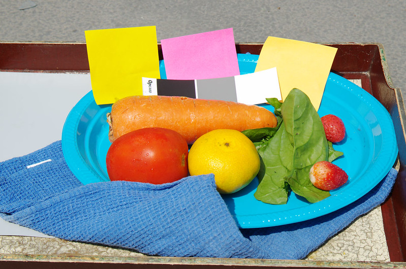
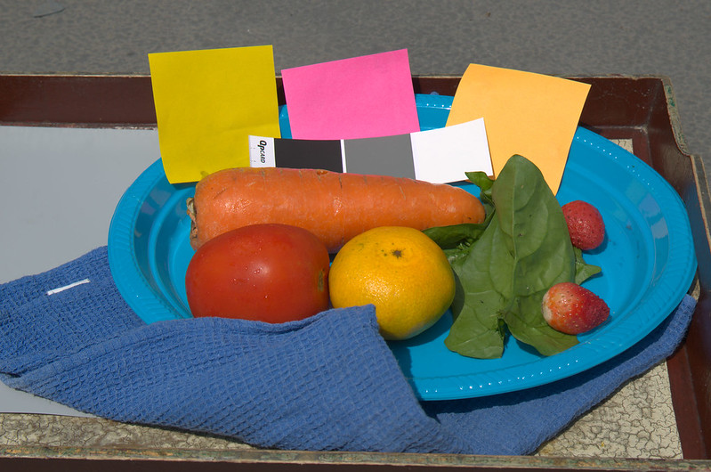
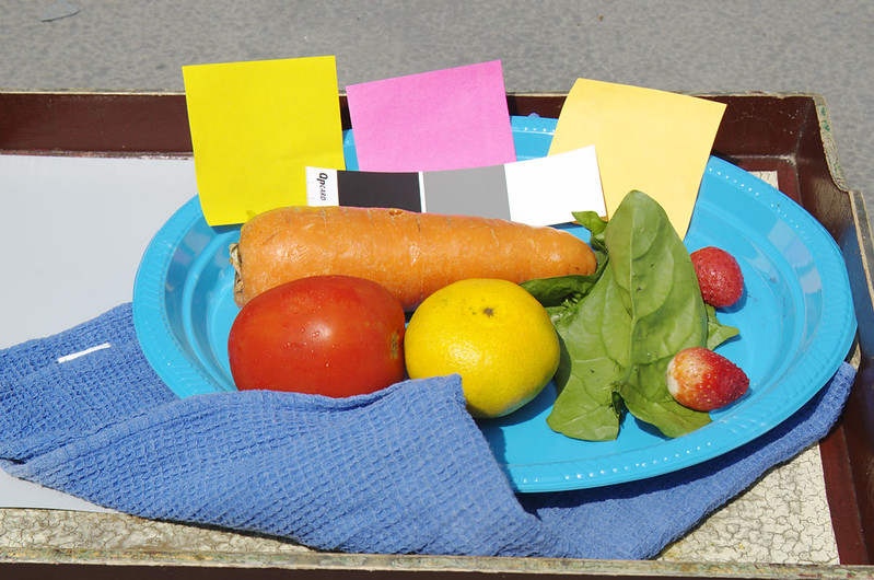
Blind test
The results from the conversion to the Adobe RGB color space —made above "by hand"— were opened in PS, and the Adobe RGB (1998) profile was assigned to them; then they were converted to sRGB to better handling of these images in the Internet browsers. A clip from them at 33.33% scale was cropped. To be sure all the images were treated exactly in the same way they were put in a stack of layers of the same PS image, including the one explained below.
Among these clips is one directly from Adobe LR V5.4 with zero settings (all default values, zero noise reduction and zero sharpening) with Adobe Standard camera calibration. This image was white-balanced using the gray patch (like those processed "by hand"), exported as Adobe RGB 16-bits .tif file, converted to sRGB, reduced at 50% to match the scale of our images without demosaicing, and then reduced additionally to 33.33% in the stack with the other images.
Below the following images is the description of each processing. Please rank them according to your taste and then check below so you can know how they were processed.

