Taking photos in RAW file format has become a ubiquitous piece of advice for any serious digital photographer. A few years ago, only DSLR cameras would bring you the chance to get RAW photos, but this is such a great feature that now, even point-and-shoot cameras are supporting RAW. Moreover, if the RAW format is not natively supported, there is even hacking software allowing to get RAW photos from cameras not officially supporting it. There is also a relatively new camera type called MILC (Mirrorless interchangeable-lens camera) also supporting RAW photos, and the list keeps growing.
In the same line, there is now much more software support for the development of photos in raw format, with great free open source options like RawTherapee, offering even better features than proprietary commercial software.
There are many good posts out there explaining why you should shoot in raw and the pros and cons about it. Knowing that National Geographic photographers shoot exclusively in raw format tells you something about the goodness of taking photos in that format.
Here we are going to show you how to develop a raw photo "by hand" instead of by using a software product. We are not suggesting this as an alternative to develop your photos on a regular basis, but as an exercise to:
- Take a glimpse of what the raw image processing software has to deal with.
- Have a hands-on experience with raw files and understand the many subjects around it.
- Have a way to get what indeed your camera produces without the effects of what your developing software introduces.
- The Tools We Will Use
- What contains a RAW file
- A Simple Plan
- Strategy to Get the Three RGB Colors per Pixel
- The Photo we Will Develop
- Extracting the Raw Color Channels
- Building (incorrectly) our First RGB Image
- Gamma Correcting our (first) Image
- Why Did We say it Was an Incorrect Attempt?
- The Strange Case of Pinkish Highlights
- Building Correctly our RGB Image
The Tools We Will Use
In this exercise we will use:
ImageJ: An image processing and analysis tool written in Java. This tool is free and very useful to manipulate images in various ways, with a lot of powerful plugins. Here you will find our introduction to ImageJ explaining the features we use here.
Iris: An astronomical image processing software (astrophotography) developed by Christian Buil. Here you will find our introduction to Iris explaining the features we use here.
RawDigger: Is a tool to visualize an examine raw data, with histograms and statistic information (like minimum, maximum, standard deviation, average) about the whole photo or rectangular samples.
If you want to replicate this exercise and you are not familiar with Iris or ImageJ, we strongly encourage you to use the links we have provided above.
What contains a RAW file
The term RAW is not an acronym; it is just an indication the image file contains —almost— non-processed sensor data. Neither it is a specific file format, there are many raw file formats, for example, Nikon® and Canon® use their proprietary raw file format, each one with a different internal structure.
The Sensor
The sensor of a digital camera corresponds to what a frame of film is for an analogical camera. A digital sensor is composed by photosites (also called photodiodes, photosensors, photodetector or sensels), where each photosite corresponds to each pixel the developed photo will contain.

Digital sensor showing its photosites
There are at least two kinds of sensors used by most of the digital cameras: the Bayer CFA (Color Filter Array) and the Foveon®, where the Bayer type is the most commonly used. For example, all Nikon and Canon cameras use the Bayer type sensor.
In the Foveon sensors, every photosite can decompose and measure the light hitting it in the red, green and blue components.

Each Foveon photosite can measure the amount of red, green and blue light hitting it. Image source: www.foveon.com
In the Bayer CFA sensor, each photosite can measure the amount of a single primary color component of the light that hits it; In other words, each photosite is sensitive only to one primary color component in the light and the other two are lost. In general, the primary colors on a Bayer sensor are Red, Green and Blue (RGB).
In a Bayer type sensor, the distinct color sensitive photosites are usually arranged in a 2x2 pattern repeated all over the sensor surface. Currently, all Nikon® and Canon® D-SLR cameras use this type of sensor. However, there are variations to this pattern, for example in Fujifilm® X-Trans® sensors the photosites follow a 6x6 pattern. There are also Bayer type sensors with photosites sensitive to four colors, like CYGM (cyan, yellow, green and magenta) or RGBE (red, green, blue and emerald).
There are two types of rows alternating along the height of the sensor: a row alternating red and green sensitive photosites, followed by another row alternating green and blue sensitive photosites. Because of this design, the quantity of green photosites is twice as red or blue ones.

Each Bayer photosite can only measure the amount of one of the red, green or blue components of the light hitting it. Image source: en.wikipedia.org
In this exercise, we will use a raw photo taken with a Nikon D7000. In that camera, the photosites are (starting from the top left corner) red and green in the first row (R, G1) and green and blue (G2, B) in the next row, precisely as in the image above. We can represent this pattern with the term GRBG, where the first G corresponds to the green sensitive photosite in a "red row" (the one containing the red and green photosites), and the last G corresponds to the green photosite in a "blue row." In some sensors, these green photosites, from the red and the blue rows -by design- do not have the same sensitivity, aiming for better accuracy of the final image. In this exercise, we will assume they have the same sensitivity. However, being able to access the raw data, we can —in the future— run some statistical tests and find if, in fact, they have the same sensitivity!
A regular non-raw picture file, like in a ".tif" or ".jpg" format, built on the RGB model, save the red, green and blue primary color components of each pixel in the image, which once they are mix reproduce each image pixel color. Notice that this mixing occurs in our human visual system (in digital devices at least) because in those displays each primary color is rendered next to the other to form a pixel.

A micro detail of an LCD pixel (emphasized with a mask), showing its primary colors. As we are unable to discriminate these pixel components, our visual system makes the mixing, and we perceive the pixel as having a single solid color.
The additive mix of the primary color components (RGB) of each pixel brings each pixel color in the image. Each pixel RGB component value represents the intensity or brightness of each primary color as part of the mix of the pixel color. For example, for one yellow spot in the color image, the red and green components —for a pixel in that spot— have relatively higher values than the blue, because you get yellow from the addition of red and green with little or no blue in the mix.
Three layers, one for each primary color, is a standard way to model this; where each layer has the whole image dimensions, but it contains only the red, green or blue (RGB) values of each pixel. With this arrangement, when the software is going to draw the color of a pixel, on a given position of the image, it reads that position from each RGB layer to get the pixel RGB color components.
Each of this RGB layers is an image on itself, but as they contain information for one color only, it usually is displayed in a monochromatic way, with higher brightness to higher component values.
However, in a raw file, there is only one layer for the whole image. Each pixel on this layer represents the light metering from each photosite in the sensor, so the first-pixel value corresponds to the reading from the red sensitive photosite, the next pixel corresponds to the green one and so on, according to the Bayer pattern we saw before. As you can see, for each pixel there is only one RGB component value, and the other two are missing.
As there is only one layer in the raw file, you can represent it as a monochromatic image. However, the brightness can vary considerably from one pixel to the next one, because these neighbor pixels represent different color components. For example, a pixel in a reddish spot, has a relatively higher value than the green and blue neighbor pixels with lower brightness, just because a reddish color has little or nothing of blue and green. This characteristic makes the distinctive appearance of the raw files when visualized with monochromatic colors, as shown in the following picture.

Strawberry detail in a raw photo image (3X). The image is shown (above) in grayscale and (below) using the color corresponding to each photosite. Notice the grayscale is a better choice.
The Units of Pixel Color values
The pixel color values in a raw file are technically dimensionless quantities. However, often they are expressed as in ADUs (Analog to Digital Units, a "dimensionless unit"). This naming is about the component in the sensor called Analog to Digital Converter (ADC), which converts the electric charge, produced by the hit of the light in each photosite to Digital Numbers (DN), which is another "unit" used for the raw pixel color values.
In the case of the Nikon D7000 raw file we will use, we will work with 14-bit ADU values. However, the 12-bit format is also usual for raw images.
In general terms, in a n-bit raw file, there are 2n possible ADU values, ranging from 0 to 2n - 1, where higher values represent higher brightness. e.g. 12-bit raw files can contain pixel color values from 0 to 4,095 ADUs, and 14-bit raw files can contain pixel color values from 0 to 16,384 ADUs.
When we say the limit for n-bit values is 2n - 1 we are not giving any "magical" formula. This limit is common sense if you understand where it comes from as we will see.
If we say we will use 3-digit decimal numbers, we can say they will have 103 - 1 = 999 as the upper limit. But when we talk about 3-bit values, we mean 3-digit values when expressed in base 2, so the upper limit is 23 - 1. Do you see the analogy? The two is in the position of the 10; we just changed the base in the formula.
A Simple Plan
As we said in the previous section, a regular RGB image is built from three layers with the same dimensions of the final image but containing the values for the RGB components of each image pixel. With the help of Iris, having those layers (as monochromatic images) is enough to build a regular color image which at the end can be saved in ".jpg" or ".tif" format, among others. So, the plan is to build the red, green and blue layers from the information in the raw file and then we will merge them to get our RGB image.
Strategy to Get the Three RGB Colors per Pixel
If in a raw file, we have information for only one RGB color value per pixel, there are two missing colors per pixel. The regular way to obtain them is using raw photo development software (either in-camera firmware or in desktop computer application). This software interpolates the colors around each photosite to compute —or rather to get an estimated value— the missing colors. This procedure is called de-mosaicing or de-bayering.
There are many demosaicing algorithms, some of them are publicly known or open source, while others are software vendor trade secrets (e.g. Adobe Lightroom, DxO Optics Pro, Capture One Software). If you are interested, here you have a comparative study of some demosaicing algorithms.
In this exercise, we will not make the demosaicing. That is something we cannot do "by hand." Instead, we will do something called binning: we have already seen how any 2x2 pixel bin in the raw file contains information for the three RGB channels. Two for the green channel one for the red and one for the blue one. So, we can imagine each bin as corresponding to a virtual photosite metering the three RGB channels at the same time. For the green channel we will average the two green readings in the bin.

The 2x2 binning will downscale each dimension by a factor of 2.
Through the 2x2 binning we will get an image with all the RGB components per pixel. However, the cost of this is to lose resolution and get an image with each dimension downscaled by a factor of two. Notice that an actual demosaicing adds the two missing color components for each raw pixel without changing the image dimensions.
The demosaicing algorithms are —of course— not perfect and may introduce some artifacts in the final image, for example they can blur parts of the image, show some edges with color fringing (false coloring) or very pixelated edges (looking like a zipper: Zippering artifact), show isolated bright or dark dots, show false maze patterns, etc.

Demosaicing Artifacts Examples: From the top left clip going clockwise: (a) maze artifacts in a rather flat sky, (b) color fringing, (c) zippering in the white diagonal plank and bright green spots, (d) Aliasing on concentric circles.
By avoiding the demosaicing, we will get an image that can be used as a reference to compare to various "real" demosaicing algorithms. We can use that comparison to tune the parameters of a demosaicing algorithm or to determine if those demosaicing algorithms introduce any unwanted features into the image. Since proper demosaicing preserves the original resolution of the raw image, it would first be downscaled by a factor of 2 to be fairly compared to our 2x2 binned version.
The Photo we Will Develop
The photo we will develop was taken with a Nikon D7000 using this Sigma 17-50mm f/2.8 lens. The aperture was f/11, with 1/200s of exposition time, ISO 100, handheld, and with Vibration Reduction (or Optical Stabilization in Sigma terms) turned on. The target is directly illuminated by the sun at 10:22 AM. The raw file format is "14-bit Lossless Compressed Raw" and is named _ODL9241.NEF with 19.1 MB of size.
The picture has "formally" 4,928 x 3,264 pixels. We say formally because physically we will find raw data for an image of 4,948 x 3,280 pixels. Probably, this is because the pixels close to the borders have not enough neighbors to make the interpolation, so 10 pixels at both vertical ends and 8 pixels at both horizontal ends do not count for the final picture when using regular development software.

This is the photo we will develop.
The photo we will develop is shown above. This image was produced with Adobe Lightroom 4.4, using the default settings but adjusting the White Balance by picking the gray patch behind the carrot.
In the following image you can click on the headings (e.g. "Log-Linear Histogram") to see the corresponding picture.


The histograms above are about the raw photo data, not from the resulting image. That's why there are two green channels. By looking at them, you can see the scene brightness range barely fits in the whole 14-bit ADU range of the file format using almost all the camera dynamic range.
The Log-Linear (logarithmic vertical scale and linear horizontal scale) at first glance seems to show substantial shadow clipping, but that is just an effect of the horizontal scale trying to show too much data in very little space. We can notice that by looking at the statistics at the right of each histogram, it is not possible such shadow clipping because the minimum values do not even reach zero.
In my camera, I have the setting for exposure control steps established at 1/3 of EV, so setting the exposure one notch below would result in ADU values downscaled by 2(1/3) = 1.26 (at least theoretically). This way, the minimum value would be 15/1.26 = 12 and the maximum 16,383/1.26 = 13,003 (approximately). However, I prefer a very little highlight clipping —without loss of any significant detail— than lowering the exposure a notch (Exposure to the right: ETTR).
Extracting the Raw Color Channels
To simplify the handling of files in Iris, in the "File > Settings : Working path" field, set the folder path where your raw-file is and where you will save the intermediate files we will produce. Let's call this the Working Folder.
You can now load the raw file in Iris by using the menu command "File > Load a raw File". In my case, I load the raw photo file "_ODL9241.NEF". Once you load the image, outside of the photo image borders, you will find one or more borders which don't seem to be part of the image. In my Nikon camera, I get that border on the right side; this is the "Optical Black" (OB) area.

Optical Black (OB) area
The pixels in this area on the raw image contain the readings of masked photosites. These photosites have a dark shield over them, so the light cannot hit them. They are used to determine the relative zero in the reading of the other regular photosites.
In some cameras (e.g., Canon) the black level is a value that you must subtract from the regular pixels (non-OB pixels) values and is either a value to compute from these OB pixels or a known value of the camera model. For example, if the value in a regular green pixel is 6,200 and the average black level in green pixels is 1,024 (either known or computed) the value of the pixel to be used in the development of the photo would be 6,200 - 1,024 = 5,176.
In the case of Nikon camera raw files, the black level is already subtracted from the photosites values, so we will use those values directly. As you can see, the raw data is not truly raw!
We are going to use the Iris Command Window, which is a way to be able to use a lot of Iris commands not available through the application menus. You must click the command button on the toolbar to open the command window as is shown in below.

Opening the Iris command window
If you hover the mouse cursor above the top right corner of the image, just before the OB pixels, you will see the coordinates x:4948, y:3280 on the Iris status bar. That's why to get rid of the OB pixels for this Nikon camera we use the "window" Iris command:
>window 1 1 4948 3280
This command will clip and keep the image from the corner (1,1) to (4948, 3280). Now you will notice the OB pixels are gone.
Now, we need to extract the "four channels" from the 2×2 binned image. The Iris command "split_cfa" collects the pixels in the 2×2 Bayer pattern and save them as images:
>split_cfa raw_g1 raw_b raw_r raw_g2
The four parameters raw_g1, raw_b, etc. are the name of the files where Iris will save the pixel color values from the 4 pixels in the 2x2 Bayer pattern, those files will have the .fit name extension. Those files are saved in the Working Folder we set at the beginning. For the GRBG pattern in the Nikon D7000 camera, the parameter raw_g1 stands for the green pixels in "blue rows", raw_b for the blue pixels, raw_r for the red pixels and raw_g2 for the green in "red rows". To load one of the green "channels" you can use:
>load raw_g1
Check how the size of the resulting image is the half of the original raw file.
You can use the sliders in the Threshold control to fit at your taste the brightness and contrast of the image. Notice that by doing that you will not change the pixel color values. Sometimes Iris automatically set this control for a "better" representation of your image. To see what you exactly have in your picture, you should use 16383, 0 in the Threshold control.

At this point you must have something like this in Iris. Here we are looking at the green channel.
Now we have two "green channels" saved: raw_g1 and raw_g2. In your working folder, you will find the files "raw_g1.fit" and "raw_g2.fit" among others. We would just use one of them and discard the another, but instead, we will take advantage of having two green readings to use the average of them (pixel by pixel), this will soften the noise in the green channel:
>add_mean raw_g 2
>save raw_g
Finally, we have the three primary colors of our binned image. They are in the files raw_r, raw_g and raw_b (with ".fit" implicit name extension).
Building (incorrectly) our First RGB Image
We can merge our three RGB channels from the raw file to build an RGB image by using the command:
>merge_rgb raw_r raw_g raw_b
Voilà! There we have our hand-developed RGB photo!! (first try). As the pixel color values in the image go from 0 to 16,383 (14-bits data), for a fair representation of the image we should use those values in the Iris Threshold control.

This is the image you get by merging the RAW color as RGB channels.
But wait, this picture is too dark, with a green/cyan color cast (look at the white patch behind the carrot). It doesn't look like the image developed with Lightroom we saw before.
There are two reasons for this situation, one is a White Balance issue (the issue is indeed something more than just White Balance, but for the moment, let's deal with it as it were only that) and the other reason is the lack of Gamma Correction in the image.
White Balance
Opening our raw channels ("raw_r.fit", "raw_g.fit" and "raw_b.fit") with ImageJ, we measure the average RGB values in the white patch (on the card behind the carrot), as described here. The mean RGB values approximately are (7522, 14566, 10411).
We can see this patch does not have a neutral color; the three RGB values should have the same value: In the RGB model, the neutral tones —those corresponding to shades from black to white— have the same value for the three RGB components.
As the white patch is the brightest area in the picture, let's scale the lower color values to match the greatest one. We will multiply the red and blue components, of the whole picture, by the required factors to make match the RGB averages on the white patch. In this sense, the required WB (White Balance) factors are ga/(ra, ga, ba) = (ga/ra, ga/ga, ga/ba) where (ra, ga, ba) are the RGB averages measured on the white patch. This is equal to 14556/(7522, 14566, 10411) = (14566/7522, 14566/14566, 14566/10411), so the WB factors are (1.936, 1, 1.399).
You should notice we are not sure if using these WB factors we will blow off-scale some color value. To be sure of that, we must find the maximum value in each RGB channel. Using ImageJ like when we measured the mean RGB values of the white patch, we will obtain the maximum values are (16383, 15778, 16383). We would also find the same values by just looking at the statistics on the right side of the raw-data histograms shown above.
As 16383 is our raw-data maximum value, we don't need any additional information to realize that any factor above one will blow up the red and blue channels, because their maximum values are both at the upper end of the scale! So, we need to adjust our RGB factors in a way their relative value still holds. Which means multiplying all of them by the same factor, and that factor must give us red and blue WB factors below or equal to one. That means we must divide them by the maximum of the red and blue WB factors max(1.936, 1.399) = 1.936. That way, our final WB factors are (1.936, 1, 1.399)/1.936 = (1, 1/1.936, 1.399/1.936) = (1, 0.5165, 0.7226).
We use this WB factors to White Balance our image using the Iris menu command "Digital Photo > RGB balance..." and we get the following image.

This is the image we get by 1) merging the RAW color as RGB channels and 2) White-balancing the white patch behind the carrot.
The cyan-blue cast is gone! But we are not there yet; the picture is still too dark.
You can notice the relative brightness of some parts in the image has changed. As we have lowered the green and blue values, the cyan/near-cyan colors are darker (green + blue = cyan). For example, look at the sky-blue plate and the rag on top of it; the same has happened with neutral colors.
Multiplying the RGB channels is a 'poor man' way to color balance the image. In a real image editing software, a full-fledged color balancing algorithm would change the pixels chromaticity but not their luminance. We will see those concepts in following sections.
Linear Brightness
The RAW file image is expected to be photometrically (this is equivalent to radiometrically but referring to EMR in the visible spectrum) correct. What this means is that the pixel values are linearly proportional to the intensity of the light that hit each photosite. In other words, if in one first spot of the sensor, the amount of light that hit the photosites was double than the amount of light in a second spot, the pixel values in the first spot would be twice as the pixel values in the second one.
This characteristic is also called linear brightness, and you need the pixel values this way for most of the image processing. This is because when a mix of colors and lights hits our retina it is radiometrically correct and we process that in what we perceive. To mimic that, the manipulation of pixel values must be done in linear scale.
However, RAW file images pixel values are not always linear for every single camera. There are standard tests to find the response of a sensor corresponding to known levels of luminance (which is the relationship we want to be linear), the result is a curve called OECF (Opto-Electronic Conversion Function).
For some cameras, this chart shows a very linear response and for others not so much. In the site of the German company Image Engineering you can see the following OECF charts for the Canon 7D and Nikon D7000.

OECF charts from a Canon 7D (left) and Nikon D7000 (Right). Source: Image Engineering. Retrieved Jan-2017
When the OECF is not linear, you must pre-process the (not so) raw pixel values with the inverse of this function to get the actual linear values. Fortunately, the Nikon D7000 we are using has a reasonably linear response.
Nevertheless, the human vision has a nonlinear perceptual response to brightness, and paradoxically when it is linear, it is not perceived as such.

The top strip has linear brightness while the bottom one is sRGB Gamma Corrected.
A Linear Perception of brightness occurs when the amount of change of the perceived brightness keeps the same proportion to the corresponding variation of the brightness values. For example, in the image above, the top strip has linear brightness increasing along the horizontal axis. This way, —for example— at one half of its length, the shown gray tone is 50% linear gray. However, you will perceive a higher change from black (0%) to 50% gray than from 50% gray to white (100%). So, the 50% gray does not correspond to our perceived middle point between black and white. Instead, it seems like the dark tones are clumped to the left end. We don't see the linear scale as linear!
The human eye perceives linear brightness changes when they occur geometrically. We can detect two patches has different brightness when they are different in more than about one percent in the linear scale. In other words, our perception of brightness is approximately logarithmic.
Gamma Correction
To correct the "clumpiness" of the black tones to the left in the linear scale; we need to use a Gamma Correction. The bottom strip also has the brightness increasing along the horizontal axis, but in this case, the tones are sRGB Gamma Corrected, and the perceived brightness changes more gradually. It appears now (more) perceptually linear and the 50% gray now seems more likely the middle point between black and white.
Notice that this does not mean the change of the image tones, it is just like converting the units we use to encode (or measure) the gray tones from linear to Gamma Corrected while preserving the perceived tones (like a unit conversion from Kilograms to Pounds). In the strips above, the 21% linear gray is converted to 50% sRGB gray; the 50% linear gray to 74% sRGB gray, and so on.
When the pixel values are linear, and our display has no way to know it, very probably will interpret them as sRGB Gamma Corrected tones. Our last image looks dark for that reason; Iris doesn't know our pixel values are in linear scale and it renders them as sRGB-Gamma-Corrected) tones. What happens here is that a gray tone at 10% in the linear scale is drawn as the gray at 10% in sRGB, a 20% linear tone as 20% sRGB, and so on. You can see (in the stripes above) this implies to draw darker tones than what the pixel values mean. This mistake is like having weights values measured in Kilograms, and someone incorrectly interpreting them as Pounds.
After the Gamma Correction, the picture will look less dark, and many people will mistakenly conclude that Gamma Correction is meant to fix some inherent darkness in linear images. When as we have seen, the picture is the same, there is only a pixel values unit conversion to allow the correct image rendering.
You might wonder if this is like converting the gray tone measurement unit, why it is not made just with the use of a simple scale factor like in 1 Kg = 2.2 lb? The issue here is the tonal scale "is closed," it starts with black (0%) and ends with white (100%). Because of that, to expand the dark tone values, we need to "gain space" by compressing the light ones. That causes the need for a Gamma Correction function instead of just a scale conversion factor, even when this is precisely just a scale conversion.
Considering the linear brightness is not perceptually linear, most RGB color spaces include a Gamma Correction.
In the Gamma Correction model, the input is linear brightness, with values from 0 (black) to 100% (white) and you must apply it to each RGB color component. The output is the gamma corrected (non-linear) brightness also in the [0, 1] range. The Gamma Correction is a power function, which means the function has the form y = xγ, where the exponent is a numerical constant known as gamma (this is the function: x raised to gamma). The very known sRGB color space uses approximately a 2.2 gamma. However, even when it is said "the gamma is 2.2" the value for the gamma term in the formula is 1/2.2, the reciprocal of the referred value and not directly the value itself.
Mathematically speaking, the gamma correction in the sRGB color space is not exactly a power function, you can read the details here in Wikipedia, but numerically speaking, it is very close to the function we saw above with a 2.2 gamma.

Gamma Correction function (blue colored curve). At lower input values, the curve has a very steep slope, expanding broadly the darkest shades. Starting from 23.6%, the slope is slowly less steep.
The correction dramatically stretches the darker tones to higher values. For example, a brightness of 10% is corrected up to 35%, that behavior goes until 23.6% which is mapped to 52%. Then the lighter tones are compressed, and the correction moves less and less those values, like 80% which is relocated to 90%.
Gamma Correcting our (first) Image
With Iris we can convert the pixel values in our first image from linear to a 2.2 gamma which is very close to the one used by the sRGB color space.
To make this conversion Iris will first scale the 14-bit pixel values from the [0, 16383] ADU camera range to [0,1]; which is the required input range in the Gamma Correction model. As the correction keeps the results in the [0,1] range Iris will have to scale them back to the [0, 16383] range:
$$ pixelValue = ((\frac{pixelValue}{16383})^{(1/2.2)}) \times 16383 $$
To follow how the gamma correction is applied, we hover the mouse cursor over the gray patch (the middle one behind the carrot) and find the pixel values are around (1516, 1530, 1527). When the Gamma Correction is applied, these values should change to (5553, 5576, 5571).
To apply the Gamma Correction, we can either use the gamma command, as shown below, or we can use the menu option "View > Gamma adjustment...". We choose the command because it allows better precision when specifying the gamma value.
>gamma 2.2 2.2 2.2
After triggering the gamma command, we hover the mouse cursor again over the gray patch and find in effect values around what we expect (5553, 5576, 5571).
For a good display of the image, we must set (16383, 0) in the Iris Threshold control, to get what we show in the following picture. Now our picture looks much better but has too little brightness contrast and looks flat.

This is our first try. We built the image RGB channels directly from the colors in the raw file, then White Balance and Gamma Correction were applied. However, the image still looks dull for the lack of color saturation and brightness contrast.
We can give the final touches to our image, enhancing its color saturation and brightness contrast, using the Iris menu options "View > Saturation adjustment..." and "View > Contrast adjustment...":

Saturation Adjustment.

Contrast Adjustment. We want more tonal separation between shadows and highlights.
After these adjustments, we finally get the following image.

This is the final version of our first try after saturation and brightness adjustments.
Compared to our previous result, this image is very much better. However, the colors are not OK yet. For example, the spinach leaf has an unsaturated green color, and the tomato is a little too dark. But as a first try, with very few steps, it is almost acceptable.
In the picture below, we can move the slider and compare, at a pixel level, our image with the one developed with Lightroom (LR). To allow a pixel by pixel comparison, I have enlarged our image by a factor of 2. By default, LR applies a sharpening filter to the image. Considering that, to allow a fair comparison, I have also added some sharpening to our picture using Photoshop (Amount:78%, Radius:2.4, Threshold:0).
Comparing side by side the pictures -as expected- there is much more detail in the LR version (we have lost resolution by the 2x2 binning). The colors in the LR version are more realistic than ours, but perhaps a little bit over-saturated and their carrot (in the right background) seems a bit too reddish.

This is a pixel level comparison of the image obtained with Lightroom (left side) and our first try of developing 'by hand' the raw photo file (right side).
Why Did We say it Was an Incorrect Attempt?
At the beginning of our first development try, we said we were doing it wrong. We said that because we treated the RAW image colors as if they were sRGB colors: we put the raw pixel color values directly in the sRGB image. Even if both the camera RAW and the sRGB use the RGB model they are different RGB color spaces, in the same way that Adobe RGB and ProPhotoRGB are different color spaces.
You cannot use the RGB color component values in one space and plug them directly in another. This very similar to having two different coordinates systems to define the position of a point. It is the same point, but it has different coordinate values in one system than in another. You must transform the coordinates of the point from one to the other.
We will understand more clearly this issue after some definitions.
Color, Light, and SPD
I think it is funny to realize the colors are just a human invention, they really don't exist as such. The colors are a human categorization of their visual experience.
We call light to the electromagnetic radiation band between approximately 300 and 700nm (nanometers: 10-9m) of wavelength: the visible spectrum. The light that comes to our eyes, has a given mix with relative power for each wavelength in the visible spectrum, which is called Spectral Power Distribution (SPD). When the SPD has a dominant power presence of waves close to 450 nm we call it blue (or bluish), when the dominant waves are close to 515 nm we call it green, and so on with each color we can see.

The visible spectrum showing approximately the color in each wavelength.
Color Model
The RGB way of representing a color as a mixture of red, green and blue (RGB) values is one of many existing color models. A color model defines a way to (uniquely) represent a color with numbers. As an analogy let's think about how to specify the location of a point in a plane. For example, there are the Cartesian and the Polar coordinate systems: both are models to uniquely represent the location of a point in a plane. In the same sense, there are many models to represent colors, all of them requiring three values to describe a color. For example, there are the CIE XYZ, xyY, Lab, Luv and CMY color models, and the RGB is just another color model.
Some color models represent a color as the mix of other (primary) colors (e.g., RGB —Red, Green, Blue— and CMY —Cyan, Magenta, Yellow— color models). Once you have defined those primary colors and made other specifications, you will have a color space based on that model. Later we will refine this concept.
The names of all the color models mentioned above are acronyms of the names of the three values used for color representation. Three values (degrees of freedom) are enough to specify any color in any given color space. The CMYK color model, has four color components just for practical reasons. Printing with the addition of black tint has practical advantages than using merely the primaries of the CMY model (without the K), which is enough to specify a color unambiguously.
The RGB is an additive color model in the sense it creates colors by adding mixes of their primaries to the substrate (screen), which is black when no primary has been added and white when all the primaries are at 100% in the mix. In contrast, a subtractive color model, like the CMY, creates colors by subtracting to the substrate (canvas, page) combinations of their primaries, which is white when no primary has been subtracted and black when all the primaries are at 100% in the mix.

Color Mixings Methods
Color Space
A color space is the set of all the colors available in a given color model. In other words, the set of colors having a valid representation in that model. A color space uses a color model with additional specifications to make a specific map from a color to its color component values.
As we saw before, a color model is a way to represent a color with color component values. As an analogy, the Cartesian coordinate system is a way to represent the location (color) of a point in the space with coordinate (color component) values. However, you can place the Cartesian system origin in any place in the space and set each axis to whatever direction you want. Here, the analogy of a color-space is a Cartesian system with fully specified origin and axis directions. Only then you will have a specific map from the point position (color) to its coordinates (color-component) values. Also, for convenience, you may use a logarithmic scale on one or more axis, and this is an analogy to Gamma correction, where the scale is transformed but the point positions (color) don't change.
We can represent a color as a point using its three values as coordinates in a 3D space. In this representation, the set of points corresponding to valid colors gets represented by a solid object, occupying a space in the model system coordinates, hence the color space name. Going further, you can represent a color space in the coordinate system of another one as in the following picture.

sRGB color space in CIE XYZ coordinates. Source: Michael Horvath for Wikipedia
Some authors distinguish between absolute and relative (or non-absolute) color spaces. In an absolute color-space, the three color-component values plus the color-space (colorimetric) specification are required to define a color unambiguously. Without that specification, the set of those colors is called a relative color space.
By itself, a set of RGB color component values are a color from a relative color space. As we saw before, those values represent a mix of their color-space primary-colors, which are part of the color space specification that allows us to get the absolute colors from the relative ones.
Most color image file formats (e.g. .png, .tif, RAW) use the RGB model. Without any additional information, the color values in those files are just in a generic RGB (relative) color space and you can't exactly know what colors are meant by those color values. That is what happened in our development exercise precisely, where Iris don't know what the camera RAW RGB specification is.
When the image file includes an embedded color-profile, containing the color space specification, the color values can be made absolute. In the absence of this data, some software may give you the chance to select some well-known color-space from a list. However, very often (like web browsers and Iris) they will suppose the color values are in sRGB.
The Mother of All Color Spaces (CIE XYZ)
Over-simplifying the whole story, the color values and models we use today are very related to two "surveys," one of 10 observers and another with seven observers conducted independently by William Wright and John Guild in the late 1920’s. These "surveys" were based on the question "Give me the combination of RGB light intensities that match this color." I find fascinating how despite some technical details were different in their experiments, and so few observers were included, the results from them are almost identical.

This plot is the comparison of Wright’s RGB coordinates at every 10nm (the points) against Guild's values at every 5nm (the lines). Look how they are almost identical. Source: www.cis.rit.edu.
In the image above, the RGB coordinates are normalized to achieve $(r + g + b = 1)$, this way; they are the fraction of red, green and blue (summing 1) required to match each wavelength color. Guild's values are based on measurements at only 36 wavelengths (approximately every 10nm). The values at each 5nm were obtained by interpolation and extrapolation using graphical techniques.
Their data was averaged, normalized, and in the quest of some desirable properties, it was linearly transformed to give birth not only the CIE 1931 RGB color space, but also the CIE 1931 XYZ and its sibling the CIE xyY color spaces. These color spaces encompass the whole human vision color space. With linear transformation, we imply the tonal scales are linear, they are not Gamma Corrected.
Notice that between the originally collected data and the final published standards there are only mathematical (linear) transformations, new data was not added. Many other studies have followed, but in the literature and many websites, you’ll find the CIE 1931 XYZ color space making an appearance often.

CIE XYZ Color Space: views around the vertical Y axis. This color space encompasses all the human vision colors.
Source: Michael Horvath for Wikipedia.
In the above image, the points on the surface correspond to the deepest (saturated) colors. The Y-axis, by design, is equal to the human perception of color brightness or Luminance. Notice how the blue tones are in the bottom end of the color space (lower Y) because they are perceptually the dark tones, while the bright yellows (higher Y) are in the top end. The other two axes do not have any meaning.
The neutral colors are along the diagonal (where x = y = z), from black in the system origin (0, 0, 0) to white in the farthest point (1, 1, 1). All the color space is in the same quadrant; there are no negative values.

An intuition of CIE xyY Color Space: Every point in the XYZ color space can be projected, towards the origin, on the X+Y+Z=1 plane.
The CIE xyY color space is in part a projection of the whole CIE XYZ color space to the plane shown with a gray triangle in the image above. You can see that any point —like $( \vec S )$— in XYZ, when projected towards of the origin, intercepts the plane $( X + Y + Z = 1 )$ (gray triangle), like in $( \vec P )$.
$$ \vec P = \frac{\vec S}{(x+y+z)} $$
If we take any point $( \vec S )$ in the CIE XYZ color space and divide it by the sum of its coordinates $( x + y + z )$ we get the point $( \vec P )$ on the gray triangle. Why we can say that? Because then the coordinates of $( \vec P )$ satisfy $( X + Y + Z = 1 )$.
In the CIE xyY color space, the x and y coordinates are the projection described above, as when seen from a point in the Z axis:
$$ x = \frac{X}{(X+Y+Z)} \\ y = \frac{Y}{(X+Y+Z)} $$
The Y value in the CIE xyY color space is the same (Luminance) from XYZ. You can easily calculate back the X and Z values.
$$ X = \frac{Y}{y}x \\ Z = \frac{Y}{y}(1-x-y) $$
This projection contains the whole human vision Chromaticity space. We will use in the following section.
Chromaticity
You can describe a color through two main components: Luminance and Chromaticity. For example, we can imagine one image projector showing a scene on a projection screen. If we vary the light beam intensity or move the projector closer or farther to the projection screen (while keeping the image on focus), we will see how the brightness of the projected image will vary. The colors will change in Luminance, while other color quality will stay equal, that is the Chromaticity.
As we know a color specification needs three values to be uniquely specified, our color decomposition in only two elements (Luminance and Chromaticity) seems to be missing something. What happens is the Chromaticity is a bi-dimensional property, you specify it with two coordinates. This way, as expected, we define a color uniquely using three coordinates: two for its Chromaticity and a third for its Luminance.

Showing the chromaticity on the CIE xy Chromaticity Space is customary.
Source: Wikipedia.
The diagram above depicts the CIE xy Chromaticity space. It contains all the chromaticity the human eye can see. The horseshoe-shaped border is called the "spectral locus," and it is marked with wavelength values from 400 to 700nm. Points on this border correspond to pure monochromatic light of the indicated wavelength.
The bottom straight line border is the locus of purples. A single wavelength cannot produce them, they represent mixes of light with wavelengths at both ends of the visible spectrum, so they are called "non-spectral.".
Any point inside the border represents a color of mixed wavelengths. The color at (1/3, 1/3) represents the CIE XYZ 'E' white reference chromaticity, which means a mix of wavelengths according to the E illuminant SPD. Later we will see more about white point/reference e illuminants.
In the previous section, we saw how we could build this Chromaticity space by projecting each color in the CIE XYZ color space towards the origin, over the $( X+Y+Z=1)$ plane.
If you take a line from the CIE XYZ surface to the origin of coordinates, every point on that line has the same chromaticity but with its Luminance diminishing as it gets closer to the origin (Y decreases).
CIE Lab Color Space
We have seen the CIE xy Chromaticity Space contains the whole human chromaticity. However, as the CIE XYZ color values are linear, that color space and its sibling CIE xyY are not perceptually uniform. Perceptually uniform means that the distance separating two colors keeps the same proportion to the perceived difference between them.

MacAdam tolerance ellipses.
Source: Wikipedia.
The picture above shows the MacAdam ellipses (ten times their actual size) showing colors within the same perceivable tolerance. If the color space were perceptually uniform, the ellipses would be circles with the same size. Two greenish colors have to be far more apart than the bluish ones to perceive the same degree of difference.
The CIE Lab color space (a.k.a. L*a*b*) is a non-linear transformation of the CIE XYZ color space (also containing the human universe of colors) having as color components the Lightness and the Chromaticity in the a-b plane. All the color components in Lab are Gamma Corrected for perceptual uniformity. Lightness is just the Gamma corrected Y Luminance from the CIE XYZ space. The used Gamma is (1/3), which is very convenient because then the 18% middle gray (in linear scale) used by photographic cameras corresponds to a Lightness of 49.5%, almost exactly in the middle of the Lightness scale. Notice that this middle gray is at 46.6% (119, 119, 119) in sRGB, just somewhat below of the desired 50%.

Projection of the CIE Lab color space on the a - b chromaticity plane, with simulated colors at about 50% Lightness. At the right end the CIE xy Chromaticity space is rotated and somewhat distorted for an easier comparison with the CIE Lab Chromaticity space.
The a axis goes approximately from green to red and b from blue to yellow. The chromaticities at the ends of a and b, in the color wheel, are at opposite sides, and those for a are perpendicular to those for b. These are called opponent channels because the color at each axis is the antagonist to the other, an equal mix of them goes to neutral, there are neither "greenish red" nor "yellowish blue" colors.
At the right end of the picture above we have included a rotated and somewhat distorted CIE xy Chromaticity Space, to help you visualize how it is transformed in the Lab Space. The green area is compressed, and the reds and purples are stretched.
Even when Lab is far more perceptually uniform than the XYZ and xyY color spaces, it turned out to be not as perceptually uniform as intended, especially in the saturated regions. Nonetheless, it is still the space used to compute color difference, but the original distance between color points in Lab space as a measure of perceivable color difference has evolved to other formulas to address its non-uniformities.

The CIE Lab color space in 3D views.
Source: Michael Horvath for Wikipedia.
The neutral tones are in a vertical line at the origin of the a - b coordinates, with white at the top (100% Lightness) and black at the bottom (0%).
Color Gamut
Color Gamut is the subset of colors that can be represented in a given circumstance, as within a color space, the colors a camera "can see", or those that an output device can show. The color gamuts are used to compare them with each other or with the whole human vision gamut.
It is very informative to compare two gamuts represented as 3D objects in a color space. However, that requires an interactive mechanism to examine the objects or the key views to allow the reader to see the differences.

Comparison of AdobeRGB 1998 (larger) and sRGB gamuts: (1) In xy Chromaticity plane. (2) In Lab a-b Chromaticity plane. (3) In Lab (3D) Space.
In the pictures above, you can see at the left (1), that both AdobeRGB and sRGB have the same chromaticities for their blue and red primaries, and only differ in the green one. You can notice this in the xy (1) and ab planes (2). However, the Luminance of the red primary is higher in AdobeRGB (29.7%) than in sRGB (25.8%), and that makes room for more luminous reddish colors in AdobeRGB than in sRGB, which you can notice at the right side of pictures (2) and (3).
You can avoid, the practical difficulties of showing gamuts in 3D spaces, with gamut projections either on the CIE xy or the Lab a-b chromaticity planes. However, in these planes, the comparison is not made between gamut spaces but between their chromaticity gamuts.

The ProPhoto (bigger) and Adobe98 RGB color spaces in Lab coordinates. Notice how in the left (chromaticity) view, the ProPhoto space seems to contain Adobe98 entirely. Nevertheless, the right picture shows some colors in Adobe98 are not in ProPhoto. These Adobe98 colors are out of the ProPhoto gamut because the blue ProPhoto primary has a very low Luminance (0.01%) and Adobe98 not so much (6.6%).
The gamut comparison in a chromaticity plane can be misleading because a third dimension is missing. You will get a wrong conclusion in cases when the difference between the gamuts is in colors with the same chromaticity but with different Luminance (the missing dimension) as in the above example.
White color, White Point, and Illuminants
White is the color we perceive when we see a material —that does not emit light by itself— reflecting with equal power all the light wavelengths striking it, and the white point of an illuminant is the chromaticity of a white object under that Illuminant. In simple words, white is the color of an illuminant, and you define it by giving its SPD.
Every color space, to be fully specified, requires a white point reference or —in other words— a standard illuminant, which defines the white-color chromaticity in that color space. For example, for the CIE 1931 XYZ color space, the standard illuminant is called "E", which has Equal power for all the wavelengths in the visible spectrum. In a diagram of wavelength-power (y) versus wavelength (x) this is a flat line. E is an ideal (hypothetical) illuminant conceived by the CIE looking for some desired numerical properties in the color space.
Sunlight and skylight compose the daylight. Depending on the balance of these components, the daylight can be relatively a bit more reddish or bluish. Regarding this fact, neither there is a single White color nor a single CIE standard Illuminant characterizing daylight illumination, but a series ("D" from Daylight) of them.
The CIE illuminant D65 is intended to portray the average noon daylight, coming from diffuse skylight without sunlight, similar to an overcast sky. According to the CIE, it "is intended to represent average daylight". On the other hand, the illuminant D50 characterize direct sunlight. Between those illuminants, the D55 portrays the average sunlight with skylight. There is also the illuminant D75 portraying the "North Sky" light.
The CIE D illuminants are very commonly used, for example, the Adobe RGB and the sRGB color spaces use the D65 as reference white, while CIE Lab uses D50. In fact, most of the color spaces use either the illuminant D65 or D50.
For a light emitting display, the "illuminant" is the color of its white representation, which for RGB displays is the color when all the RGB channels are at 100% intensity.

This spectrum diagram shows the relative power (SPD) of some illuminants according to CIE standards. The approximate color of each wavelength is shown in the background, this way we can see the D65 illuminant has more intensity in bluish wavelengths than the D50 which instead has more power in reddish ones.
From a realistic point of view, the CCT characterization of daylight SPD for a specific place, depends among other factors, on the date of the year, time of the day, the sky state, the site altitude, pollution and the location of the site in the world. In other words, just because the illuminant was direct sunlight, it doesn't mean the CIE illuminant D50 will accurately describe that illumination.
CCT: Color Correlated Temperature
To precisely specify a light source, we need to characterize its SPD as we do with the illuminants in the previous section image. For example, here is data describing CIE A and CIE D65 illuminants with their relative intensity for each wavelength. But for practical reasons, this is too cumbersome. Fortunately, there is a mathematical model for a theoretical light-emitting-object called ideal Planckian black body radiator, which radiates light of comparable spectrum to that emitted by natural sources.
The SPD of this ideal black body is only a function of its temperature. This way, an SPD can accurately be specified by just giving the temperature that makes this black-body emit such spectrum.

Spectral power distributions of CIE illuminant D65 and an ideal black body with the D65 correlated temperature (6504°K).
In a similar way as when we see glowing colors in an incandescent metal object, the ideal black body with increasing temperatures, shows colors hues from reddish/orange ("warm") to light-blue ("cool") hues at the higher temperatures. Notice how —ironically— "warm" colors correspond to lower temperatures and conversely "cool" colors corresponds to higher ones. The temperature is customary given in Kelvin degrees (°K). In a chromaticity space, the set of points representing the color of a black body at different temperatures, fits in a curve called "Planckian locus".
The temperature at which a Planckian Black Body Radiator and an illumination source appear to match is called the Color Temperature. Light sources with chromaticity falling exactly over the Planckian locus have True Color Temperature, while chromaticity near the locus have Correlated Color Temperature (CCT).
This is the origin of the numerical part in the series D illuminants names, it is the illuminant CCT (in hundreds). For example the CCT for D65 is 6500°K while the CCT for D50 is 5000°K.

The red curve above shows the chromaticity of CIE illuminants D50, D55, and D65 as points on the CIE daylight (D) locus and the blue curve below them shows the Planckian locus. Notice the graph scale, these curves are very close to each other. The curves are on the CIE 1960 UCS color space. Derived from: Wikipedia image.
Often, the White Balance control interface, in photo and image editing software, is based on the navigation over this space. In this sense, the control interface contains a temperature slider to walk over the Planckian locus, to White Balance the colors resulting from a scene under an illuminant with a given CCT, and a tint slider to walk perpendicular to the Planckian locus, to affect the relative green-magenta balance.

White Balance controls. In left column from top to bottom: Adobe Lightroom, DxO Optic Pro, Rawtherapee. At the right side: Capture NX2.
However, as this control is used to White Balance the effect of an illuminant with a given CCT, the effect of this slider is to tint the image with the opposite (complementary) color. This way, an illuminant with a relative low CCT, with a reddish/orangish color, is balanced with a blue color casting, while illuminants with a higher CCT, with a bluish hue, are balanced with a yellow color casting. For this reason, the temperature slider is shown with a graduation from blue to yellow, showing the hue casting that will be used to White Balance the image.
The tint slider is graduated from green to —its complementary color— magenta, showing again how it will affect the image.
For example, the White Balance control of Adobe Lightroom, DxO Optics Pro and Rawtherapee —in the image above— are based on the navigation on the Planckian locus as we described before. Rawtherapee has an additional slider based directly on the relative intensity of blue and red intensities, so there is an option to everyone taste. The Capture NX2 White Balance control shows exactly the factor that will multiply each, red and blue color components.
There are standards specifying bins along the CIE D illuminants and the Planckian locus, normalizing tolerances about when a light can be characterized with a specific CCT. For example, the ANSI C78.377A standardize the description of tints in LEDs and Solid-State Lighting.

ANSI C78.377-2008 is a standard developed by the American National Standards Institute (ANSI), the American National Standard Lighting Group (ANSLG), and the National Electrical Manufacturers Association (NEMA) in 2008 to standardize the description of tints in LEDs and Solid-State Lighting. Source: www.colorkinetics.com
The bins in the graph above, seem to get larger from left to right. However, we must remember the CIE xy Chromaticity plane is not uniform, the same distance between color points in this plane does not mean similar perceivable color differences. These bins have similar perceivable tolerance but have different sizes to counteract the non-uniformity issue.
The RGB Color Model
In the RGB model, each color is described as a mix of red, green and blue primary colors, where each primary can vary in a continuum between 0 to 100%.
When there is the same amount of the three primaries R = G = B the resulting color is neutral, from 0% for black to 100% for white.

3D representation of the RGB model. The origin is black. The diagonal line represents the mix of the same amount of each primary, rendering shades of gray from black to white.
When a spot on a RGB display has one of its primaries at the 100% and the others are at 0%, the spot will show the purest or deepest possible color corresponding to that primary. For example (r:0, g:100%, b:0) will show the deepest possible green on that display. As the display can only show colors based on the combination of its primaries, the depth of all the colors it can produce is limited by the depth of its primaries.
The RGB color model is like a "template" of color spaces, the absolute specifications of the primary colors are required —and the white reference as for any color space— to have an absolute color space. That's why there is one RGB color model but there are many RGB color spaces: Adobe RGB, Apple RGB, CIE RGB, ProPhoto RGB, sRGB, etc.

Comparison of Adobe RGB and sRGB gamuts. Adobe RGB has a larger gamut, basically to accommodate colors with deeper green. Image derived from Wikipedia.
The chromaticity of the colors a RGB output device can produce is limited by the chromaticity of its primary colors. This can be clearly seen on the CIE xy chromaticity space shown in the image above, where each triangle vertex marks the chromaticity of each primary color, and each triangle surface represents the set of chromaticities the corresponding color space can represent. The borders of the triangles correspond to the deepest colors available on each space.

This is an RGB color space, projected —towards the origin— over the diagonal plane R + G + B = 1. You can imagine this triangle, transformed into the xy space, like the one you see in gamut comparisons on that chromaticity plane.
To have an intuition of how a triangle in the CIE xy chromaticity plane can describe an RGB space chromaticity, you can imagine each color point in the RGB space projected towards the origin and intercepted by the diagonal plane (R + G + B = 1) as in the image above. This triangle converted to the CIE xy space is what we see in RGB gamut comparisons on that space.
The sRGB color space is a very well-known standard, which is assumed by many applications, including web browsers, as the color space of an image when there is no information describing its actual color space.
8bit RGB displays
From a practical point of view, we must consider the RGB displays (e.g. CRT monitor, LCD or LED flat screens, cell phones, tablets, iPad, TV, and so on) nowadays use 8 bits per RGB channel (if not less, as all modern analogue and even most digital video standards use chroma sub-sampling by recording a picture's color information at reduced resolution).
This means, the RGB displays can only show 256 intensity levels for each primary color, this is 2563 = 16.78 million of colors, a lot of them!. It doesn't matter if you are watching on your screen computer an image coming from file with 16-bit per channel (e.g. a 16-bit ".tif" file). For display purposes, the image data will be linearly quantized to a maximum of 256 values per channel.
For example, in the development exercise we are doing, the specular reflections on the sky-blue dish, show in Iris status bar RGB coordinates around (16383, 15778, 16383). With a threshold control set with (16383, 0), this is shown in the screen as (16383, 15778, 16383)*255/16383 = (255, 245, 255).
Color Profile
From a practical point of view, the color profile is a file associated to an input or output device, containing the required information to transform —absolute— color coordinates to/from the device color space. In the first case it is referred as input color profile and in the second as output color profile.
Let's suppose we have a scanner as input device and a color printer as output device. At a low-level layer, the scanner and printer native color spaces do not match, it is required to translate colors form one space to the other. To make the things simpler and get a more useful solution to this situation, the concept of input color profile is to convert the input device color coordinates from its color space to a universally known one, as CIE XYZ or Lab (so called profile connection space), and the output profile takes the colors from that connection space and takes them to the output native device native space. This is like two guys with different native language using two interpreters translating from one native language to English and another from English to the other native language. However, the color profiles are data, information specifying how to make those translation, they are not code or software.
Only with this information, an application can accurately represent colors in/from the device. When this information is not available for a screen (output device), the software applications may assume the device color space is equal or at least very close to the sRGB color space. In this circumstance -when the device has not a known color profile- the accuracy of the colors in/from the device depends on how close its actual color space is to the sRGB.
For general use, there is mainly two kinds of color profiles, the Adobe DCP (DNG Camera Profile) and the icc color profiles. As you might guess the DCP is an input profile while the icc profiles can be prepared for input or output devices.
What is the matrix?
Unfortunately, no one can be told what the Matrix is.
You have to see it for yourself.
Very often, when working at a low level with colors, it is required to use a color matrix. This matrix essentially represents the transformation of one color point coordinates from one space to another. I know, this starts to sound like a complicated mathematical subject, but don't worry, we will deal with it as a notational subject, we want you to know from where everything comes from.
Let's suppose we have the (x, y) coordinates of a point P with respect to the system XY and we want the coordinates (u, v) with respect to the system UV.

The coordinates of the point P are (x,y) and are given with respect the system XY, we want to obtain the coordinates (u,v) with respect to the UV system.
If you look at the diagram above you will notice we can compute u by adding and subtracting the length of some line segments. In particular we can get u this way:
\begin{align*} u &= \overline{OB} - \overline{AB} \\ \overline{AB} &= \overline{AD} - \overline{BD} \\ \Rightarrow u &= \overline{\textbf{OB}} - \overline{\textbf{AD}} + \overline{\textbf{BD}} \end{align*}
With the help of trigonometric functions we can find the length of the line segments we need to compute u. For example we can say:
\begin{align*} \overline{\textbf{OB}} &= x / cos(\theta) \\ \overline{PB} &= y - x \cdot tan(\theta) \\ \overline{\textbf{BD}} &= \overline{PB} \cdot sin(\theta) \\ \Rightarrow \textbf{BD} &= y \cdot sin(\theta) - x \cdot tan(\theta) \cdot sin(\theta) \\ \overline{PD} &= y \cdot cos(\theta) - x \cdot sin(\theta) \\ \overline{\textbf{AD}} &= \overline{PD} \cdot tan(\theta + \phi) \\ \Rightarrow \overline{\textbf{AD}} &= y \cdot cos(\theta) \cdot tan(\theta + \phi) - x \cdot sin(\theta) \cdot tan(\theta + \phi) \\ \\ \therefore u &= x / cos(\theta) - y \cdot cos(\theta) \cdot tan(\theta + \phi) + x \cdot sin(\theta) \cdot tan(\theta + \phi) + y \cdot sin(\theta) - x \cdot tan(\theta) \cdot sin(\theta) \end{align*}
We can see u is a linear transformation of (x,y). We would continue and get also the formula of v, but instead, we can think about those formulas at a higher level of abstraction and see that at the end, both u and v must be a linear function of x and y, like u = m1·x + m2·y + c —for some m1, m2 and c— after all, x and y are the only lengths we have, right? Besides, the coordinate systems XY and UV have the same origin, (e.g. black is encoded as (0,0,0 in RGB, XYZ and Lab) so when (x,y) = (0,0) also (u,v)=(0,0), which gives 0 = m1·0 + m2·0 + c, in other words c = 0. If we follow the same reasoning, we will get a similar formula for v, and at the end we will have something like:

In the case of colors, we use points with three coordinates, so to transform the (x, y, z) coordinates the formulas will be like:

This is the kind of formula that arises very often transforming color coordinates from one space to another, so it worths simplify its notation making explicit the matrix operation inside it:

In the above formula, as M is a matrix, the multiplication by xyz implicitly denotes a matrix multiplication, not a scalar one. This kind of matrix is often called Color Matrix. Here you will find this kind of formula to transform a color from CIE XYZ coordinates to sRGB linear coordinates, and here is used for chromatic adaptation.
When you have this matrix to transform from xyz to uvw, you implicitly have the formula for the other way around, from uvw to xyz. You just have to invert the matrix at the other side of the formula:

The matrix multiplication is not commutative, which means that in general "A×B" is not equal to "B×A".
Different Photosite Sensitivities
In a photo taken to a white object (e.g. a sheet of paper) while using white light (e.g. outdoor, directly illuminated by the sun in a clear day), we would expected the RGB values in the raw image file would have the same coordinate values R = G = B. After all, "it uses the RGB model" where the neutral colors have as RGB color components the same value. Well, that really doesn't happens at all.
If you look at the histogram of raw image data about a white object that was photographed as described in the previous paragraph you will find something like this:

These are the raw histograms of a white object in a photo. Notice how the red values are roughly the half of the green ones.
The red, green and blue sensor photosites have very different relative sensitivity, and this can be better noticed when looking at a white object in the photo. The most sensitive is the green photosite, then the blue and finally the red. This behaviour is like if the camera would have a greenish-cyan lens filter and by looking through it, a white object looks greenish and the red-wine colors has equal RGB values in raw data.

For digital sensors, colors like the red-wine at the image left side results with equal value in the raw RGB channels. It is like the green color at the right (its complementary color) were used as lens filter.
This is not a matter of sensor quality. If we look at the top of the camera sensors ranking at DxO Mark, we will find this characteristic pretty much alike in all sensor brands.
The following table shows data from that site, showing the multipliers required to apply to the red and blue raw values in order to get the level of the green ones for pixels corresponding to a white object under a CIE illuminant D50.
| Brand | Model | Red raw | Blue raw |
|---|---|---|---|
| Nikon | D800E | 2.02 | 1.49 |
| Sony | A7R | 2.52 | 1.59 |
| Phase One | IQ180 | 1.46 | 1.98 |
| Pentax | K-5 IIs | 2.10 | 1.72 |
| Canon | EOS 1Dx | 1.97 | 1.50 |
| Nikon | D7000 | 2.11 | 1.50 |
The Strange Case of Pinkish Highlights
If you see the histograms above you can imagine an increasing exposure as the shifting of these RGB peaks to the right side. In such case, —eventually— the green peek will hit first the raw upper limit (in this case 16,383 is the right end of the histograms scale) and wont be able to shift anymore to the right. All the "overflowing" green values will be kept at the upper limit of the scale, and as a consequence, all those pixels with this truncated green value will not be able to have the relative balance among their RGB components to correctly represent the photographed source color.

Raw highlight clipping with the green channel almost totally overflown.
If the raw conversion process doesn't take the right precautions, the spots on the image corresponding to this highlight clipping will show the relative absence of the green component, and they will look pinkish or magentish. This is because magenta and green are complementary colors, so the color balance will go to magenta when the green component is decreased.
In our image development, this kind of highlight-raw-clipping occurs in the specular reflections on the sky-blue dish. Before color balance, they have a raw RGB value around (16383, 15779, 16383), which is shown on the screen (multiplied by 255/16383, because —remember— RGB displays use 8-bits per channel) as (255, 245, 255) which is technically a little magentish, but it is so bright that almost looks white. After the white balance adjustment, that value changes to (1, 0.5165, 0.7226)*(16383, 15779, 16383) = (16383, 8141, 11845) which in the screen results in (255, 127, 184), looking clearly reddish/pinkish as shown in the following image.

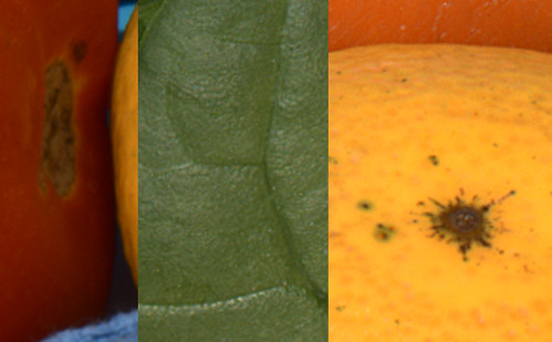
The left most clip is the image composed by raw RGB values. It is hard to see the highlight is a little magentish. White balancing the first clip results in the center clip, where the highlight is clearly reddish. The third clip is the final result after gamma correction and adjustments of saturation and contrast, there you can see the pinkish highlight.
To correct this problem, we have to White-Balance the image raw channels, find the minimum in the maximum channel values min(max(red), max(green), max(blue)) and clip the channels, in a way that at the end, all of them have the same maximum pixel value.
What we are doing with this procedure, is dealing with the raw channels as if they had pixel values with different units, and by doing the white-balance we convert them to the same pixel value unit. After this, we can compare the channels, and knowing the maximum values corresponds to the highlight, we clip them to the smallest one in order to get the same maximum value in all the channels, achieving this way neutral highlights.
In the image we are processing, the maximum raw values after white balance are (16383, 8141, 11845), so we must clip the red and blue channels to 8141.
We will use the Iris command clipmax <old top> <new max> which affects the pixels with values greater than <old top> assigning them the <new max> value. In our case, we want the values above to 8141 to have the value 8141, that corresponds to clipmax 8141 8141.
The Iris command mult <factor> multiplies all the image pixel values by a given factor. We will use this command to white balance the image, then we will clip the pinkish highlight, and finally we will reverse the white balance to get our raw channels in the original camera raw domain. This will allow us to work later with different approaches on the subject of different raw channel scales (caused by the different RGB photosites sensitivities) without the issue of pinkish highlights.
** Processing the raw Red channel **
>load raw_r
>mult 1
>clipmax 8141 8141
>mult 1
>save raw_phc_r
** Processing the raw Green channel **
>load raw_g
>mult 0.5165
>clipmax 8141 8141
>mult 1.9361
>save raw_phc_g
** Processing the raw Blue channel **
>load raw_b
>mult 0.7226
>clipmax 8141 8141
>mult 1.3839
>save raw_phc_b
When we multiply the raw channels by (1, 0.5165, 0.7226) we are white balancing the image, and when we multiply the channels by (1, 1.93611, 1.3839) we are multiplying them with the reciprocal of the factors used for white-balance, reversing that white-balance: (1, 1.9361, 1.3839) == 1/(1, 0.5165, 0.7226).
Now, we have our raw channels saved in the files (raw_phc_r, raw_phc_g, raw_phc_b) free of pinkish highlights (the "phc" term in the file names stands for "pinkish highlight corrected").
Notice how we must white balanced the raw channels as input to our procedure while building the final image. Once we have the sRGB image we can white balance it —again— this time in the sRGB space and as part of the final touches, but the different raw photosite sensitivities must be handled with white-balanced channels in the camera raw space to avoid the appearance of color artifacts.
Another interesting thing to notice, is how —in the previous procedure— we have clipped to a maximum of 8141 ADU the red and blue channels, right when they had 16383 and 11845 maximum pixel values (correspondingly), this seems a harsh clipping!. We can use ImageJ to find out the image areas affected by that clipping. The following images show how only the specular highlights are clipped, there is no loss of significant detail in the image.


Sometimes it is overlooked that image areas with shadow clipping can suffer analogue problems to those we described for highlight clipping: When there is decreasing exposure, the peaks in the histograms are like moving to the left, and it is possible that only the red channel gets clipped to 0. In a similar way to highlight clippings, if the raw converter does not take the required precautions, the dark areas —with this shadow clipping— will show a color shifting to the cyan, the red complementary color, or will look greenish if both red and blue are clipped.